Viscoelastic Homogenization with Time-dependent Constituent Properties
In this example, we want to compute the effective properties of a composite material made of isotropic viscoelastic matrix and transversely isotropic elastic fiber. The fiber properties are defined by means of engineering constants as specified in the table below.
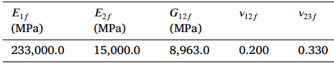 Fiber properties defined as transversely isotropic elastic
The matrix properties are given as a time-dependent properties, which means that for each time a value of the Young’s modulus is given. In addition, we will consider that the matrix has a constant Poisson’s ratio equal to 0.37. We will create a text file to input the time-dependent material properties as follows.
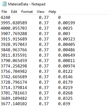 Time-dependent matrix properties
Please note that for different viscoelastic anisotropies, the material properties should be defined as follows in different columns.
- Transversely isotropic. —- Young’s Modulus, E (t) —- Poisson’s ratio, nu (t) —- Time, t
- Orthotropic defined by means of engineering constants. —- E1 (t) —- E2 (t) —- E3 (t) —- nu12 (t) —- nu13 (t) —- nu23 (t) —- G12 (t) —- G13 (t) —- G23 (t) —- Time, t
- Orthotropic defined by means of stiffness matrix. —- D1111 (t) —- D1122 (t) —- D2222 (t) —- D1133 (t) —- D2233 (t) —- D3333 (t) —- D1212 (t) —- D1313 (t) —- D2323 (t) —- Time, t
- Anisotropic. —- D1111 (t) —- D1122 (t) —- D2222 (t) —- D1133 (t) —- D2233 (t) —- D3333 (t) —- D1112 (t) —- D2212 (t) —- D3312 (t) —- D1212 (t) —- D1113 (t) —- D2213 (t) —- D3313 (t) —- D1213 (t) —- D1313 (t) —- D1123 (t) —- D2223 (t) —- D3323 (t) —- D1223 (t) —- D1323 (t) —— D2323 (t) — Time, t
We will use a square pack 2D SG with fiber volume fraction equal to vf = 0.64.
Software Used
In his tutorial we will use Abaqus CAE with the Abaqus SwiftComp GUI plug-in. Abaqus CAE will be used to GUI to define the time-dependent material properties and to run the viscoelastic homogenization. SwiftComp will run in the background.
Solution Procedure
The steps required to compute the effective viscoelastic properties using Abaqus SwiftComp GUI are as follows.
# Step 1. We define the material properties in global coordinate system. We click on Materials in Abaqus CAE and define the Fiber properties by means of the engineering constants and click “Ok”.
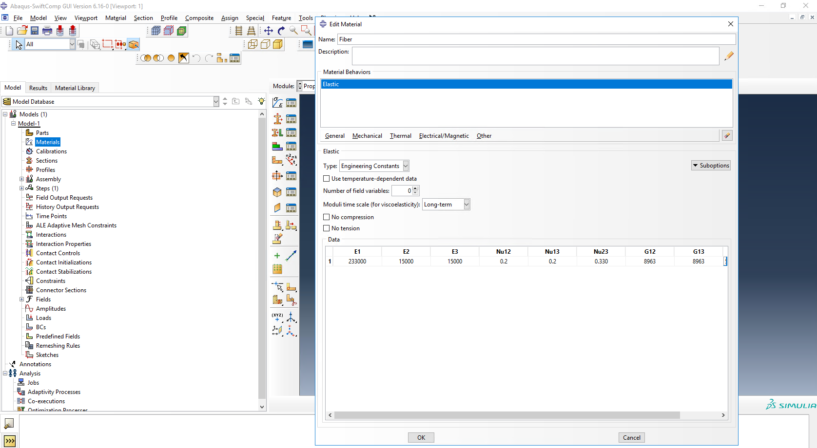 Definition of the fiber properties
# Step 2. Within the Materials of Abaqus CAE, we create a dummy material called “Matrix”. Please note that we will not define the Prony coefficients of the resin using the Abaqus SwiftComp GUI in the next step.
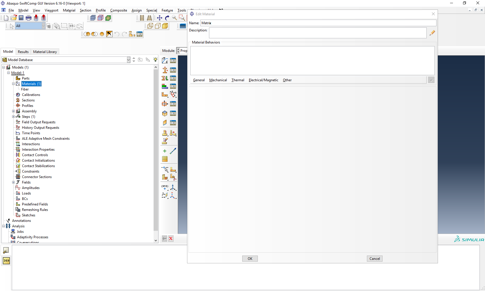 Creation of the dummy material for the matrix
# Step 3. In the Abaqus SwiftComp GUI menu, we click on Input Time-Dependent Properties. We select “Time-dependent” and “Viscoelastic” in the Method & Analysis section. We pick “Matrix” as the Material to be modified in the drop down menu. Then, we look for the text file used to input the material properties. This text file can be located in any folder of the computer. Finally, we click the two “Ok“s as shown in the picture.
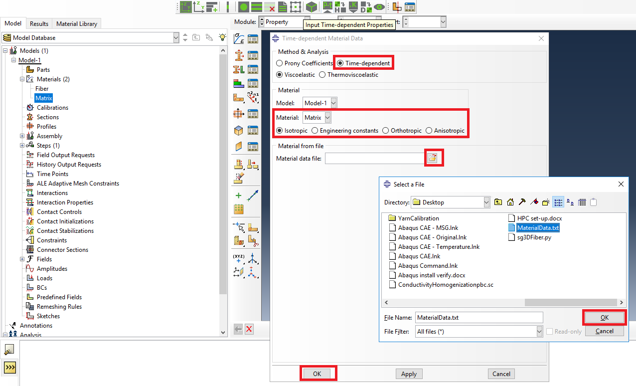 Definition of the matrix Prony coefficients
# Step 4. From the default the Abaqus SwiftComp GUI SGs, we pick the 2D Structure Genome with Square pack. We input the fiber volume fraction, define the approximate global mesh size, and click “Ok”. A square pack microstructure will be automatically generated.
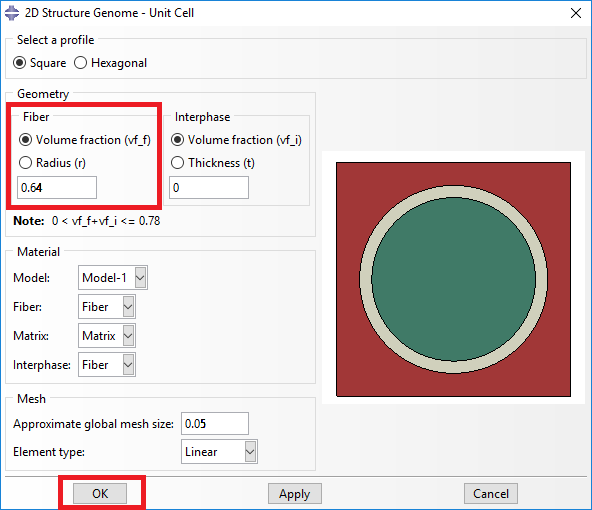 Definition of the 2D SG square pack microstructure
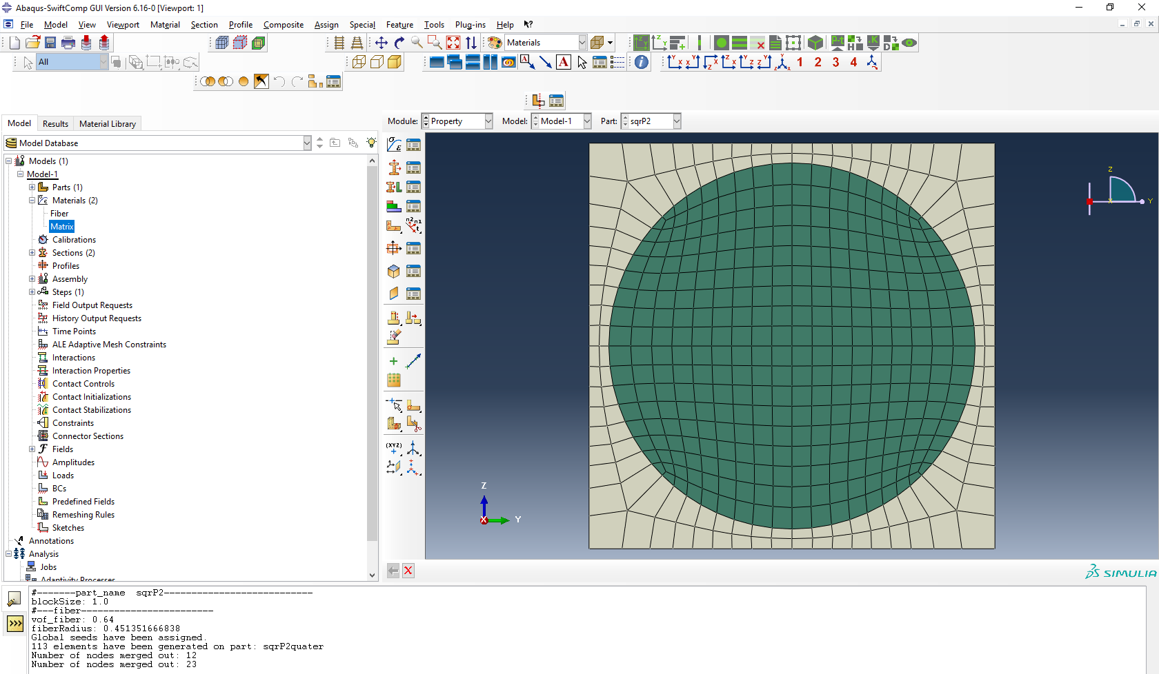 2D SG square pack microstructure
# Step 5. Now, we will compute the effective viscoelastic properties. To do so, we click on Homogenization and select Viscoelastic in Analysis Type. In the Viscoelastic/Thermoviscoelastic Analysis section, we define the range of the time (i.e. Initial time” and Final time”) in which we want to output the effective properties as well as the frequency (i.e. Time increment” defined in decades).
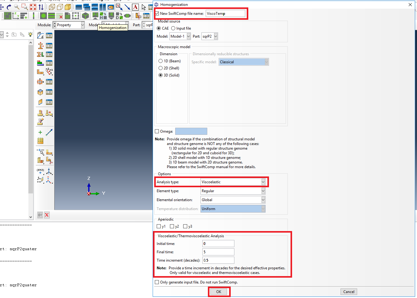 Definition of the viscoelastic homogenization step
# Step 6. We click on Ok to run the homogenization step. SwiftComp on the background will run the homogenization.
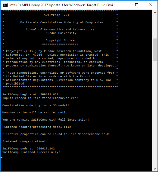 SwiftComp running on the background
# Step 7.The results can be found in the .sc.k file as shown next. Note that the effective properties will be outputted for each specified time.
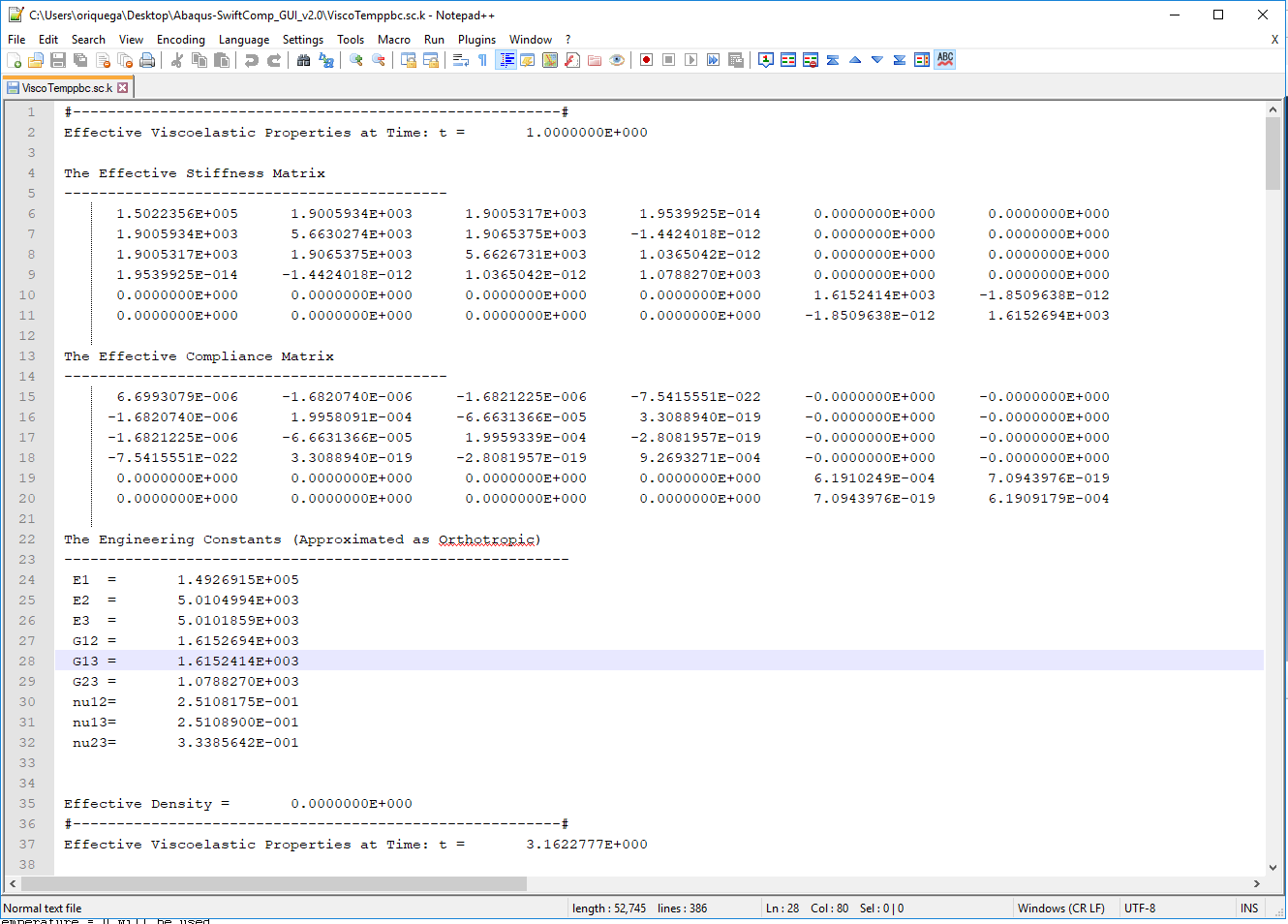 Results corresponding to the effective viscoelastic properties
References
- Liu, X.; Tang, T.; Yu, W., Pipes, R. B.: “Multiscale modeling of viscoelastic behavior of textile composites,” International Journal of Engineering Science, Vol 130, September 2018, pp. 175-186, DOI: 10.1016/j.ijengsci.2018.06.003.
- Rique, O.; Liu, X.; Yu, W., Pipes, R. B.: “Constitutive modeling for time- and temperature-dependent behavior of composites,” Composites Part B: Engineering, Vol 184, March 2020, DOI: 10.1016/j.compositesb.2019.107726.