Thermoviscoelastic Homogenization
This tutorial shows how to calculate cross-sectional properties of the Corrugated boom with given dimensions and material properties using SwiftComp 1.3 and SwiftComp Abaqus GUI.
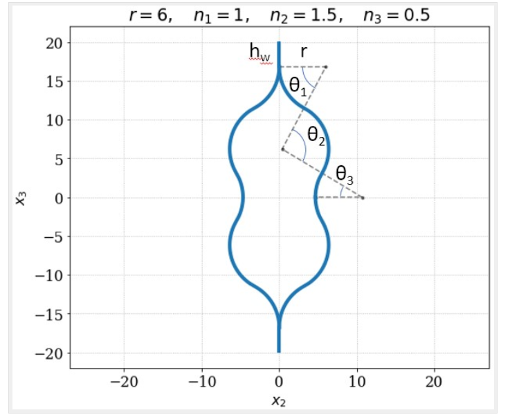
Flattened height: 45 mm, Web height(one side): 3 mm, Subtended angle: 90 degree, Ply thickness: 0.4 mm,
Radius of the flange (curved part): 6.00 mm,
Layup: (30)2 .
In this example, we want to compute the effective thermoviscoelastic properties of a composite material made of isotropic thermoviscoelastic matrix and transversely isotropic thermoelastic fiber. The fiber properties are defined by means of engineering constants and coefficients of thermal expansion (CTEs) as specified in the table below.
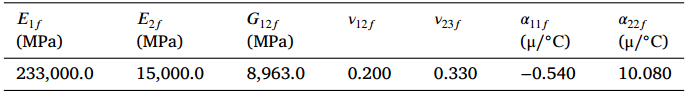 Fiber properties defined as transversely isotropic elastic
The matrix properties are given by means of the Prony coefficients presented in the table below. In addition, we will consider that the matrix has a constant Poisson’s ratio equal to 0.33 and CTE equal to 60 μ ∕◦C .
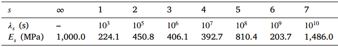 Prony coefficients and relaxation times for the matrix
We will use a square pack 2D SG with fiber volume fraction equal to vf = 0.64.
Software Used
In this tutorial we will use Abaqus CAE with the Abaqus SwiftComp GUI plug-in. Abaqus CAE will be used to GUI to define the time-dependent material properties and to run the thermoviscoelastic homogenization. SwiftComp will run in the background.
Solution Procedure
The steps required to compute the effective viscoelastic properties using Abaqus SwiftComp GUI are as follows.
# Step 1. We define the material properties in global coordinate system. We click on Materials in Abaqus CAE and define the Fiber properties by means of the engineering constants. To introduce the CTEs, we select Orthotropic” in Type section. We will also need to provide a value to the specific heat. For this tutorial, we will consider the specific heat equal to 1. Finally, we click “Ok”.
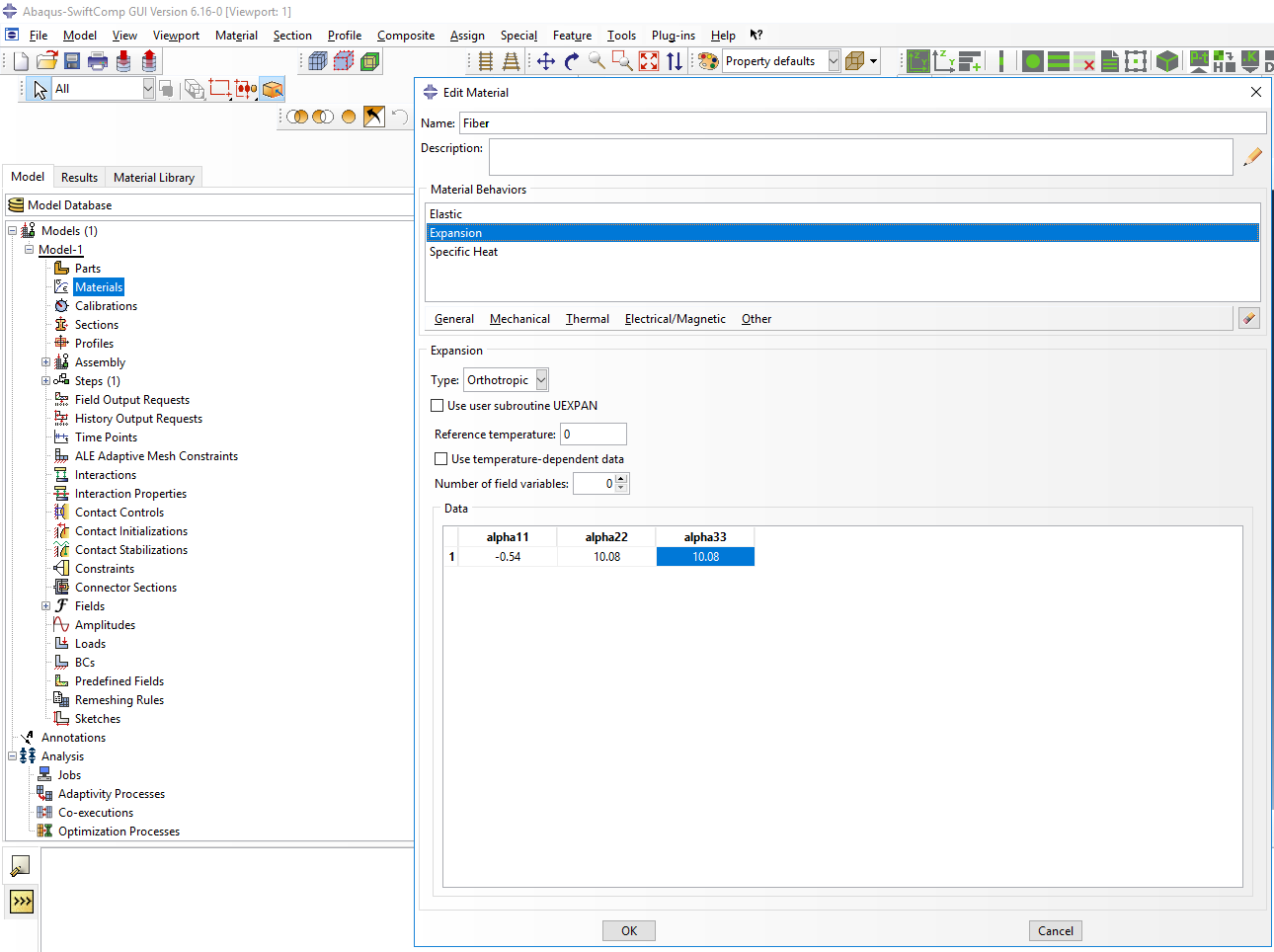 Definition of the fiber properties
# Step 2. Within the Materials of Abaqus CAE, we create a dummy material called “Matrix”. Please note that we will not define the Prony coefficients of the resin using the Abaqus SwiftComp GUI in the next step.
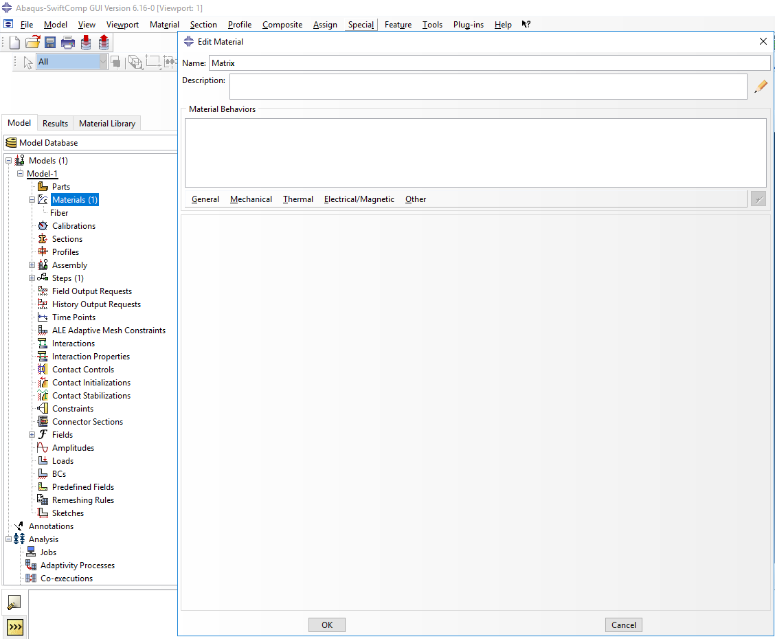 Creation of the dummy material for the matrix
# Step 3. In the Abaqus SwiftComp GUI menu, we click on Input Time-Dependent Properties. We select “Prony Coefficients” and “Thermoviscoelastic” in the Method & Analysis section. We pick “Matrix” as the Material to be modified in the drop down menu. Then, we input the relaxed Young modulus, Poisson’s ratio, Prony coefficients, and the constant CTE value. It is noted that we also introduce 0 in the Prony coefficients of the table. Finally, we click “Ok”.
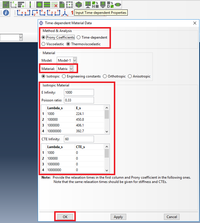 Definition of the matrix Prony coefficients
# Step 4. From the default the Abaqus SwiftComp GUI SGs, we pick the 2D Structure Genome with Square pack. We input the fiber volume fraction, define the approximate global mesh size, and click “Ok”. A square pack microstructure will be automatically generated.
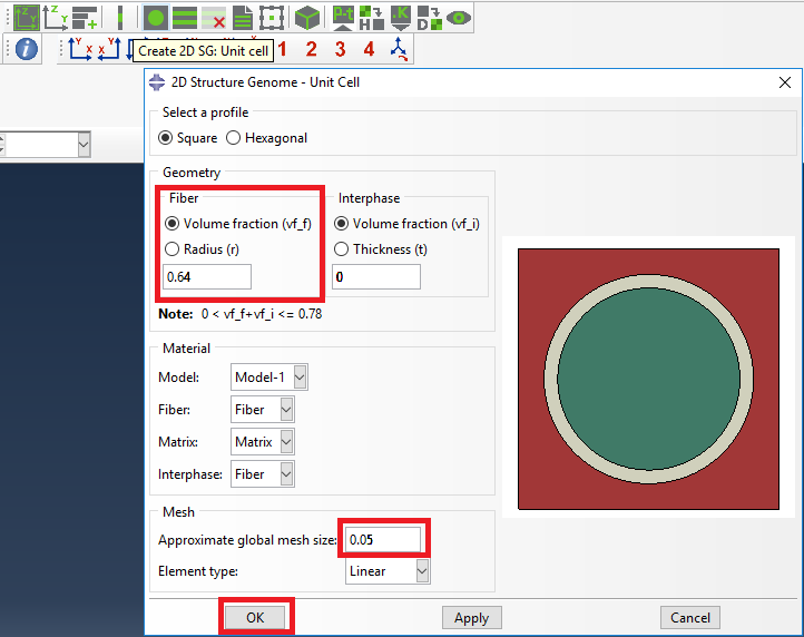 Definition of the 2D SG square pack microstructure
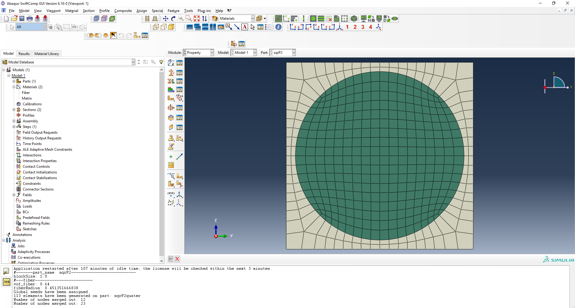 2D SG square pack microstructure
# Step 5. Now, we will compute the effective thermoviscoelastic properties. To do so, we click on Homogenization and select Thermoviscoelastic in Analysis Type. In the Viscoelastic/Thermoviscoelastic Analysis section, we define the range of the time (i.e. “Initial time” and “Final time”) in which we want to output the effective properties as well as the frequency (i.e. “Time increment” defined in decades).
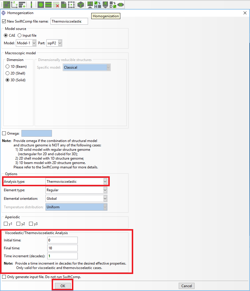 Definition of the thermoviscoelastic homogenization step
# Step 6. We click on Ok to run the homogenization step. SwiftComp on the background will run the homogenization.
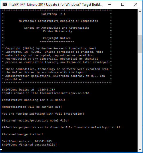 SwiftComp running on the background
# Step 7.The results can be found in the .sc.k file as shown next. Note that the effective properties, which includes the effective CTEs, will be outputted for each specified time.
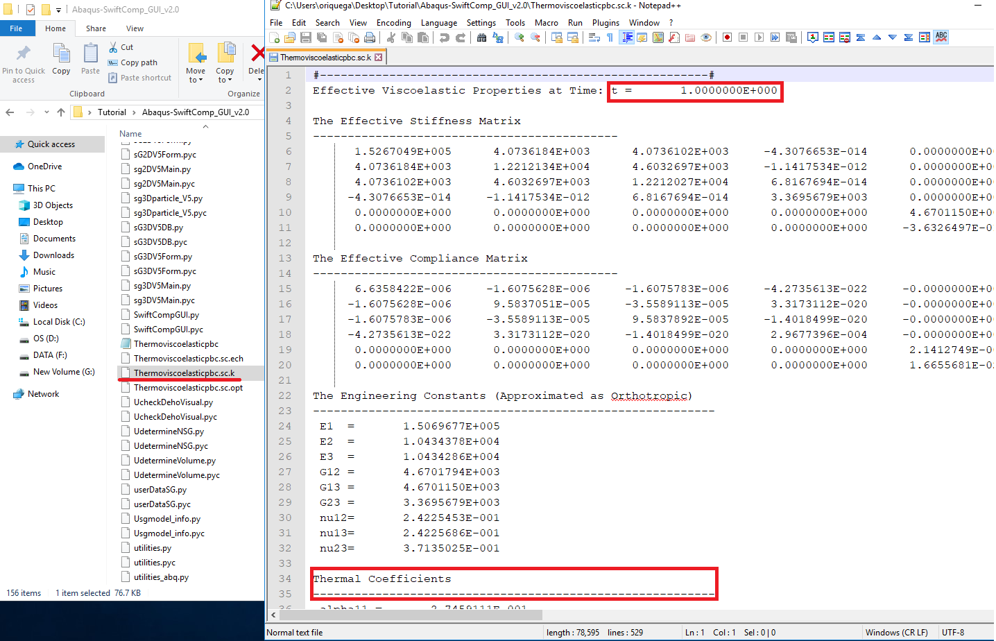 Results corresponding to the effective thermoviscoelastic properties
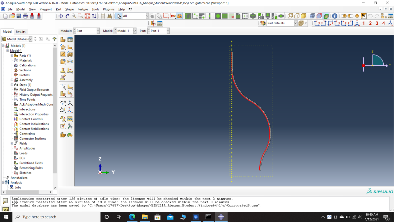
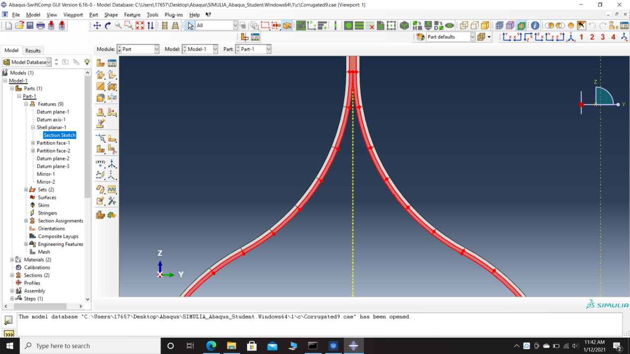
# Step 9.’Create the part geometry for the Corrugated Boom.Use Set sketch plane for customized SG (Pointed by the Black arrow) -> Use create planar shell -> Select the plane and vertical axis -> Sketch a fourth of the base line (Highlighted as a red line). Its geometry is a straight line (Web height) from (0,19.78) to (0,16.78) and three curved lines (Flange) one from (0,16.78) to (3.18,11.48) centered at (6,16.78) and another from (3.18,11.48) to (5.5,3.08) centered at (0.36,6.18) and the last one from (5.5,3.08) to (4.65,0) centered at (10.64,0). Set its thickness to 0.2 mm to the right of the baseline and partition the flange curves at around 10° intervals to obtain a smooth curve. Partition the part in the middle to obtain two plies off thickness 0.1 mm each. Mirror the part about the vertical and the horizontal to get the geometry of the Corrugated Boom.
 Layups
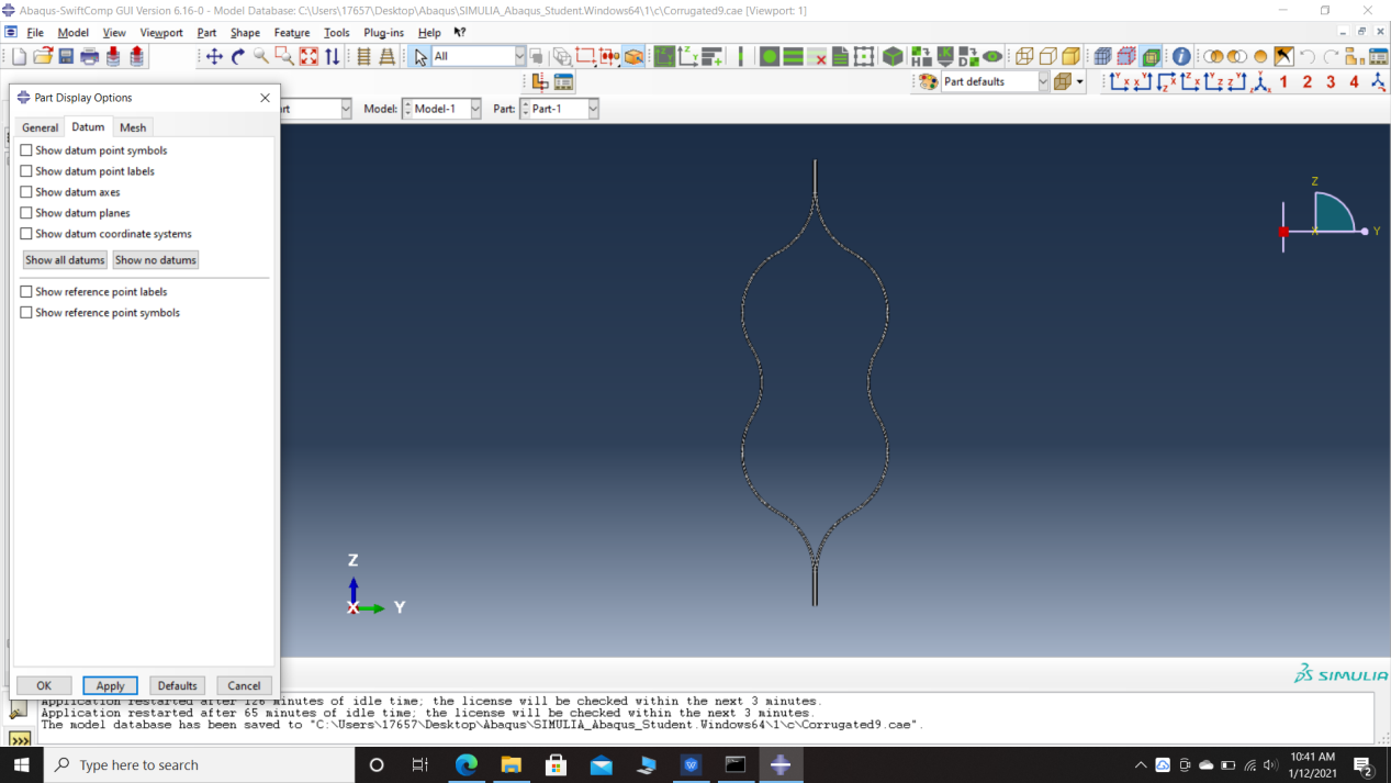 sketch plane
# Step 10.To enter the material properties for the part, first we need to manually calculate the material properties for both the plies one with orientation 45° and the other with orientation -45°. Choose the material properties from the results of the computed effective viscoelastic properties in the previous section for the appropriate time interval(As required) .Use the formula C’=Rsigma*C*(Rsigma)Transpose to obtain the rotated properties. Now we proceed to enter the properties of the part as follows. Go to Property -> Create material -> Mechanical -> Elasticity -> Elastic -> choose in Type Engineering constants and add the material properties for one of the plies. Repeat the steps for the other ply. Now create two shell homogeneous sections, each one corresponding to one of the materials using the create section option. Now assign the material properties using the assign section option as follows. Select the plies corresponding to the material to select the appropriate section after choosing done.
 Material properties
# Step 11. Module > Mesh > Seed Part and choose mesh size, then Click ‘Mesh Part’
 Mesh
Mesh
# Step 12. Homogenize the part to get the final results.
 Homogenization
References
- Rique, O.; Liu, X.; Yu, W., Pipes, R. B.: “Constitutive modeling for time- and temperature-dependent behavior of composites,” Composites Part B: Engineering, Vol 184, March 2020, DOI: 10.1016/j.compositesb.2019.107726.