Viscoelastic Beam Properties of a TRAC Boom
This tutorial shows how to calculate cross-sectional properties of the TRAC boom with given dimensions and material properties using SwiftComp 2.1 and Abaqus SwiftComp GUI.
Flattened height: Web height: 10 mm, Subtended angle: 90 degree, Ply thickness: 0.1 mm,
Radius of the flange (curved part): 25 mm,
Layup: (0/45/-45/90/0)s. The layup sequence is along with the direction pointing to the center of flange.
Material properties are given as follows:
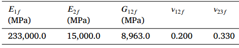 Fiber properties defined as transversely isotropic elastic
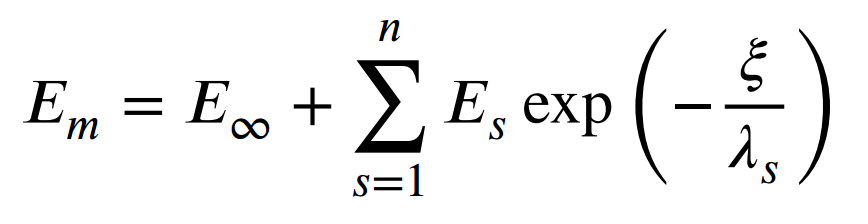
The matrix properties are given by means of the Prony coefficients presented in the table below and following the formulation of Figure 1. In addition, we will consider that the matrix has a constant Poisson’s ratio equal to 0.33.
 Definition of the Young modulus of the resin
 Prony coefficients and relaxation times for the matrix
We will use a square pack 2D SG with fiber volume fraction equal to vf = 0.64.
Software Used
In this tutorial we will use Abaqus CAE with the Abaqus SwiftComp GUI plug-in. Abaqus CAE will be used to GUI to define the time-dependent material properties and to run the viscoelastic homogenization. SwiftComp will run in the background.
Solution Procedure
The steps required to compute the effective viscoelastic properties using Abaqus SwiftComp GUI are as follows.
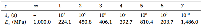
# Step 1. We define the material properties in global coordinate system. We click on Materials in Abaqus CAE and define the Fiber properties by means of the engineering constants and click “Ok”.
 Definition of the fiber properties
# Step 2. Within the Materials of Abaqus CAE, we create a dummy material called “Matrix”. Please note that we will not define the Prony coefficients of the resin using the Abaqus SwiftComp GUI in the next step.
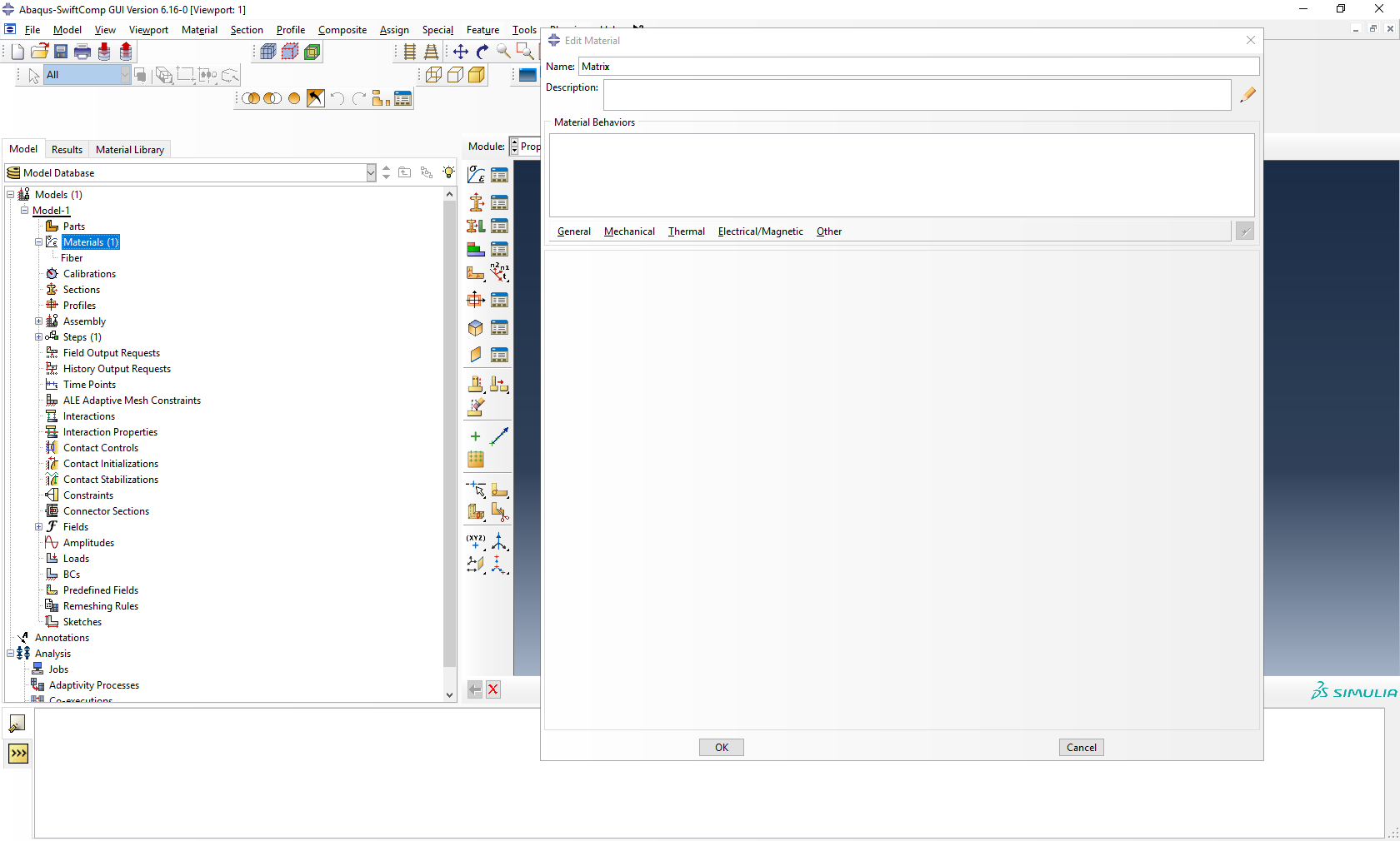 Creation of the dummy material for the matrix
# Step 3. In the Abaqus SwiftComp GUI menu, we click on Input Time-Dependent Properties. We select “Prony Coefficients” and “Viscoelastic” in the Method & Analysis section. We pick “Matrix” as the Material to be modified in the drop down menu. Then, we input the relaxed Young modulus, Poisson’s ratio and the Prony coefficients following the equation presented above. Finally, we click “Ok”.
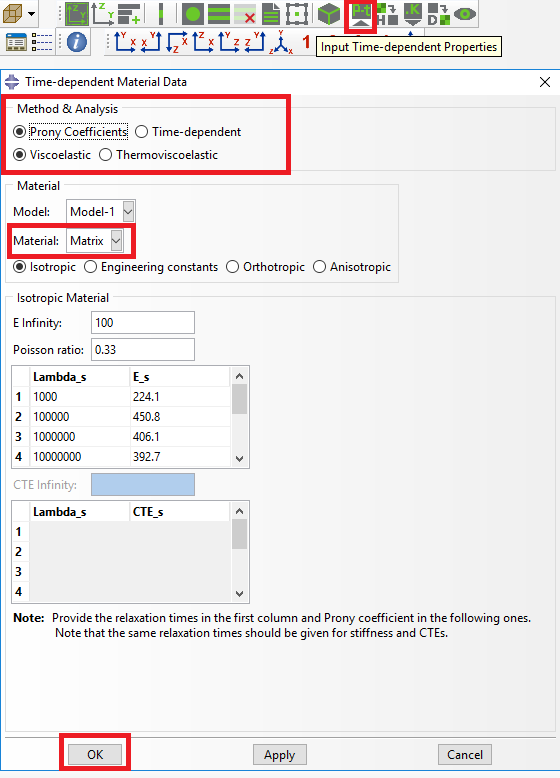 Definition of the matrix Prony coefficients
# Step 4. From the default the Abaqus SwiftComp GUI SGs, we pick the 2D Structure Genome with Square pack. We input the fiber volume fraction, define the approximate global mesh size, and click “Ok”. A square pack microstructure will be automatically generated.
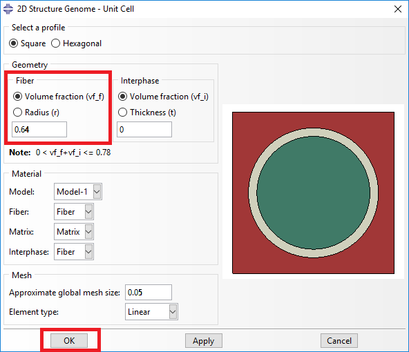 Definition of the 2D SG square pack microstructure
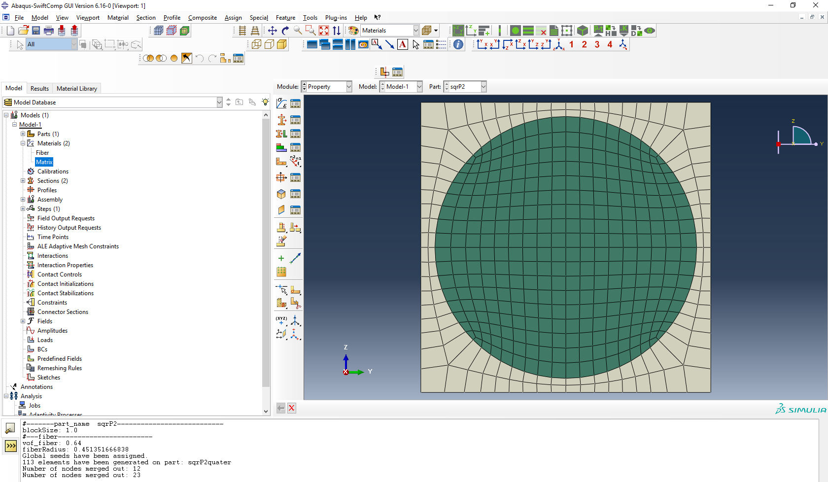 2D SG square pack microstructure
# Step 5. Now, we will compute the effective viscoelastic properties. To do so, we click on Homogenization and select Viscoelastic in Analysis Type. In the Viscoelastic/Thermoviscoelastic Analysis section, we define the range of the time (i.e. Initial time” and Final time”) in which we want to output the effective properties as well as the frequency (i.e. Time increment” defined in decades).
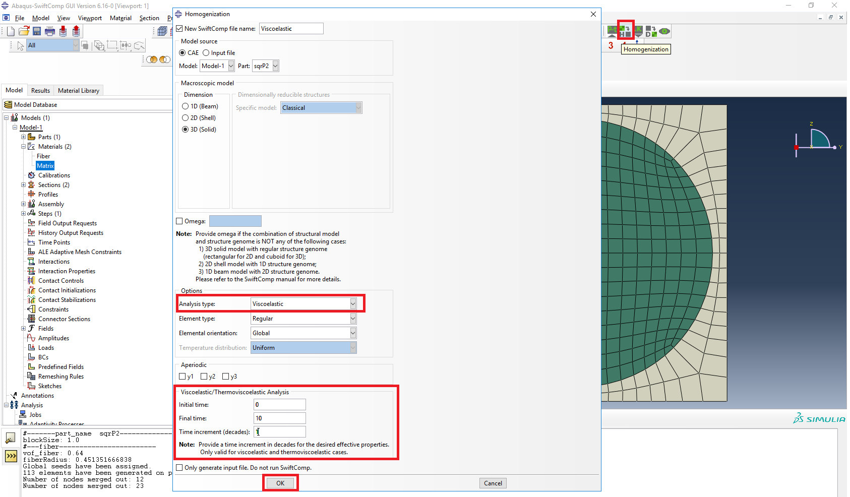 Definition of the viscoelastic homogenization step
# Step 6. We click on Ok to run the homogenization step. SwiftComp on the background will run the homogenization.
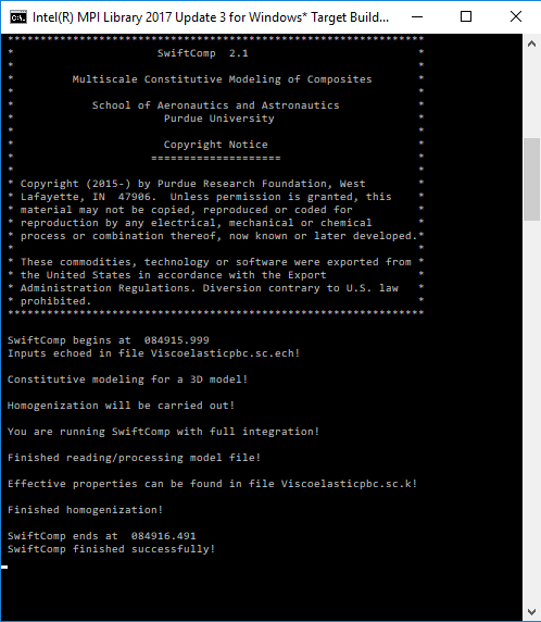 !SwiftComp running on the background
# Step 7.The results can be found in the .sc.k file as shown next. Note that the effective properties will be outputted for each specified time.
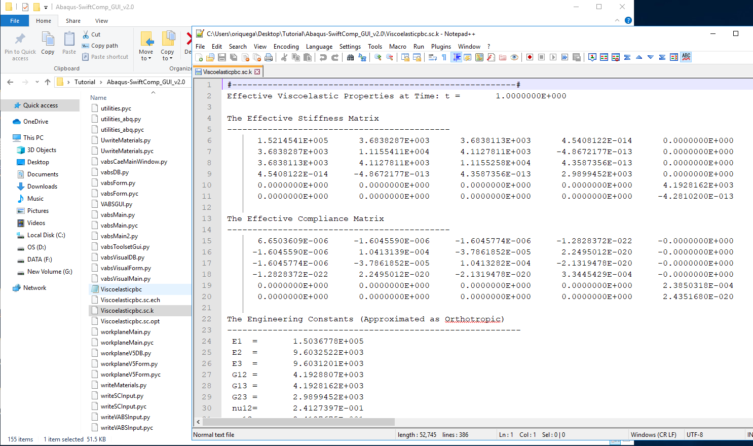 Results corresponding to the effective viscoelastic properties
# Step 8.We move on to macroscopic homogenization of the trac boom.
 Trac boom
# Step 9.’Create the part geometry for the TRAC Boom. Use Set sketch plane for customized SG -> Create planar shell -> Select the plane and vertical axis -> Sketch half of the base line (Highlighted as a red line). Its geometry is a straight line (Web height) from (0,10) to (0,0) and a curved line (Flange) from (0,0) to (25,-25) centered at (25,0). Set its thickness to 1 mm to the right of the baseline. Mirror the part about the vertical to get the geometry of the TRAC Boom. Partition the part to seperate the web and flange and also the individual flanges.
 Part Geometry
# Step 10.To enter the material properties for the part, first we need to choose the material properties from the results of the computed effective viscoelastic properties in the previous section for the appropriate time interval(As required or we can also use time depended properties as explained in its tutorial) . Now we proceed to enter the properties of the part as follows. Go to Property -> Create material -> Mechanical -> Elasticity -> Elastic -> choose in Type Engineering constants and add the material properties.
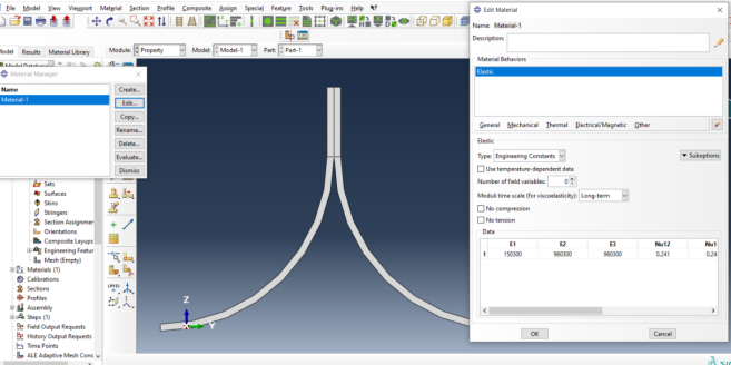 Material properties
‘ # Step 11. Now go to New Layups and add the material, section name, Layup and thickness to create the required layup. This can be repeated if we have multiple layups.
 Layups
‘ # Step 12. Now go to Create 2D SG: Assign Layups and the pick the baseline, the line opposite to the baseline and the area between the two picked line for the right flange as shown and then hit Ok. Do this for all four sections
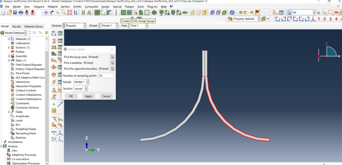 Assign Layups
# Step 11. Module -> Mesh -> Seed Part -> set approximate global mesh size, then Click ‘Mesh Part’
 Mesh
Mesh
# Step 12. Homogenize the part preferably as a 1D beam to get the final results.
 Homogenization
References
- Liu, X.; Tang, T.; Yu, W., Pipes, R. B.: “Multiscale modeling of viscoelastic behavior of textile composites,” International Journal of Engineering Science, Vol 130, September 2018, pp. 175-186, DOI: 10.1016/j.ijengsci.2018.06.003.
- Rique, O.; Liu, X.; Yu, W., Pipes, R. B.: “Constitutive modeling for time- and temperature-dependent behavior of composites,” Composites Part B: Engineering, Vol 184, March 2020, DOI: 10.1016/j.compositesb.2019.107726.