YouTube video of this tutorial: https://youtu.be/e9KOjx7kmTY
Problem Description
The MSG solid model is used to predict the effective viscoelastic properties of a plain weave composite using a two-step approach.
The first step predicts the effective viscoelastic yarn properties based on the elastic fiber and viscoelastic matrix properties at the microscale. Instead of fitting Prony series for yarn properties, SwiftComp provides another option to define the viscoelastic properties of yarns using general time-dependent properties. This will avoid the efforts in fitting Prony series and the inaccuracies in the fitting.
The second step takes the effective yarn properties and matrix properties to predict the viscoelastic properties of weave composites.
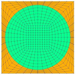
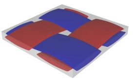
The microscale and mesoscale models are given as
Software Used
Solution
Preparation: Fiber and matrix properties organized in a .txt file
Since the viscoelastic properties are defined using Prony series or time-dependent properties, users need to input a lot of information. To simplify this process, TexGen4SC 2.0 provides a function to let users import the properties from a text file. An example of defining viscoelastic properties at the microscale is given as
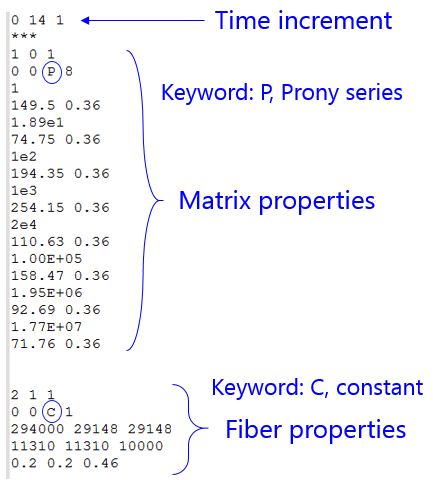
In this example, Line #1 through Line #20 are to describe viscoelastic properties of the matrix, while Line # 23 to Line # 27 are elastic fiber properties. Specific meanings of these numbers are given as below.
- Line #1: log10(start time), log10(end time), log10(time increment). Viscoelastic materials exhibit time-dependent behaviors. This line specifies the time point where you want to calculate the effective yarn properties. In this example, “0 14 1” means the time starting from $$10^0$$s to $$10^{14}$$s and the increment is $$10^1$$s. Therefore, this analysis will be performed at {$$10^0$$,$$10^1$$,$$10^2$$, …, $$10^{14}$$}.
- Line #2: separation from the time increment to the material properties as expressed using “***”.
- Line #3: material ID, type of isotropy, number of temperatures. Here, the first number “1” means material No. 1. The second number “0” means “isotropic”. This can also be “1” (orthotropic), or “2” (anisotropic). The last number “1” means one temperature considered. These are inherent descriptions used in SwiftComp to define material properties. You may find more details about description conventions in SwiftComp User Manual. The most relevant contents are on Page 29 of “SCtheory.pdf” .
- Line #4: temperature, density, type of description, number of series terms. In this case, temperature is not a variable so we leave these two as zeros “0 0”. To study thermal effects, please check other examples such as thermoelastic properties of plain woven composites. “P” stands for Prony, which means that the matrix properties are expressed using Prony series: $$E(t) = E_{inf} + sum(E_kexp(-t/\rho_k))$$, where $$\rho_k$$ is the relaxation time. Prony series expansion is a common method to describe viscoelastic behaviors by fitting experimental data with a finite number of exponential terms. “8” stands for the number of exponential terms.
- Line #5, 7, …19: $$\rho_k$$ of each term in Prony series.
- Line #6, 8, …20: Young’s modulus ($$E_k$$) and Poisson’s ratio ($$\nu_k$$) in each term. Poisson’s ratio is assumed to be time-independent in this case.
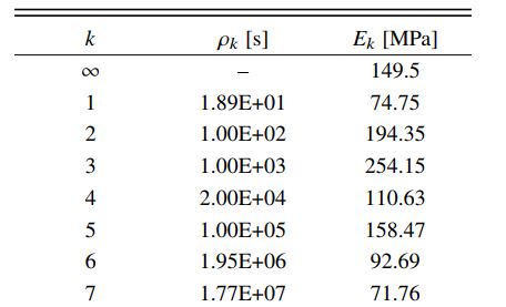
- The Prony series coefficients of the matrix are given as
- Line #23: “2 1 1” means material No. 2, orthotropic (“1”), 1 temperature. Same conventions applied here as in Line #3.
- Line #24: “0 0” as no temperature or density change. “C” stands for Constant which means the fiber properties are time-independent. “1” means one set of material properties.
- Line #25, 26, 27: for an orthotropic material (“1”), nine constants are used to describe the material. The nine constants are arranged in these three lines as:
| $$E_1$$ | $$E_2$$ | $$E_3$$ |
| $$G_{12}$$ | $$G_{13}$$ | $$G_{23}$$ |
| $$\nu_{12}$$ | $$\nu_{13}$$ | $$\nu_{23}$$ |
Now we’re ready to calculate yarn and fabric properties using TexGen. Below describes the step-by-step procedure to solve the problem. It is better to accompany this document with the youtube video.
1. Create plain weave pattern
- Click “Weave” to create mesoscale plain weave SG.
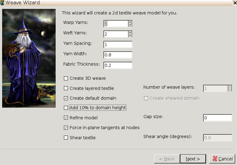
- Input the yarn geometries.
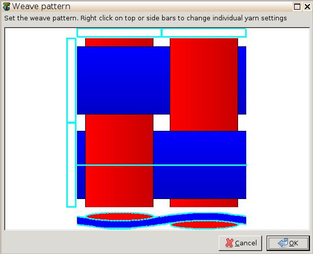
- Click “Next” and you’ll see some yarns in 0 and 90 degree directions.
- Click on the upper-right and lower-left squares to get the woven pattern.
- Click “OK”, and the correct fabric pattern will show up after several seconds.
2. Microscale (yarn) properties
- Now you need to upload the .txt file containing matrix and fiber properties to the current session (data/sessions/number).
You may use any FTP app, for example, FileZilla, to set up connection with cdmhub.org/your_user_name, and to upload and download the files.
Alternatively, in Terminal you may type in the following commands:
sftp your_user_name@cdmhub.org with your login password
cd /home/cdmhub/your_user_name/data/sessions/six_digit_session_number
put /path_to_your_local_.txt_file/filename.txt
use get command if you want to download any result file.
- Once you uploaded the .txt file, click “Microscale” under “Homogenization” tab for yarn property calculation.
- Select “Viscoelastic” as the type of analysis.
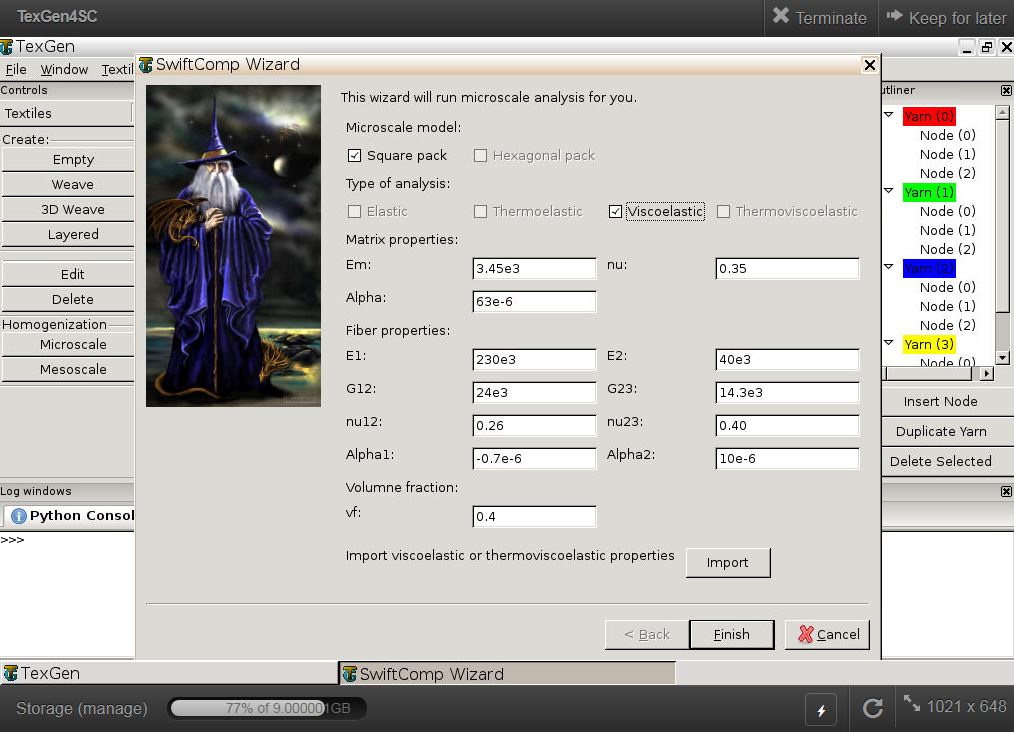
You may ignore the matrix and fiber properties in the window, as we’ll import properties from the uploaded file.
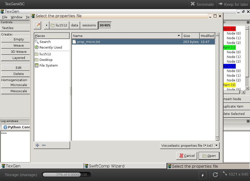
- Click “Import” and select the uploaded .txt file.
- Click “Finish”.
Now a .sc file (micro.sc) will be generated that SwiftComp will take as the input. SwiftComp will run on the cloud to calculate viscoelastic properties of yarns, e.g., effective microscale properties. In the pop-up window, you will find the analysis results.
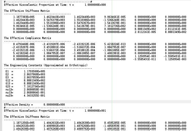
This file (micro.sc.k) is automatically saved in your current session folder. You may transfer it to your local computer.
3. Mesoscale (fabric) properties
- Go to “File->Export->SwiftComp File” to generate the .sc file for mesoscale analysis.
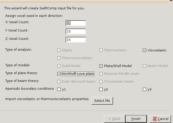
- Define the voxel mesh
- Select “Viscoelastic” as Type of analysis
- Select “Plate/Shell model” and “Kirchhoff-Love plate”
- Click “Select file” and select “prop_meso.txt”
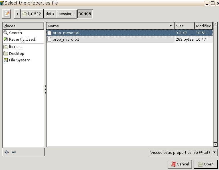
The file named “prop_meso.txt” is automatically generated during microscale analysis, and will be used as part of mesoscale analysis input file.
- Save the .sc (SwiftComp input file) file with a filename you designate.
- Click “Mesoscale” in “Homogenization” tab, which will call SwiftComp to calculate fabric properties.
You’ll get the effective ABD matrices of this single-ply plain weave laminate!
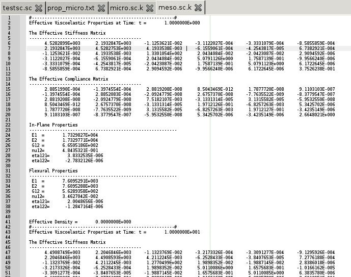
Again, you may transfer this file (“the_filename_you_saved.sc.k”) to your local computer for further analysis.
For details about the MSG viscoelastic theory, please refer to the reference paper.
References
- Liu, X., Tang, T., Yu, W. and Pipes, R.B., 2018. Multiscale modeling of viscoelastic behaviors of textile composites. International Journal of Engineering Science, 130, pp.175-186.
