Prof. Yu's Research Group in the Cloud

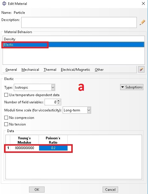
Let the material properties of the particle and matrix be: Particle-E-glass: E₁₁ =80 GPa, v₁₂=0.2000 and

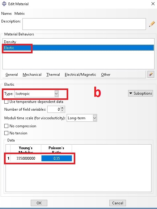
Matrix: E =3.35GP, ν=0.35

Particle volume of fraction is assumed to be 50%

The material properties are obtained from: “Soden, P. D., Hinton M. J. and Kaddour, A. S., Lamina properties, lay-up configurations and loading conditions for a range of fibre reinforced composite laminates. Compos. Sci. Technol., 1998, 58(7), 1011”
youtube link:
https://youtu.be/XdmrqaI3wtw

Step 1: Input material properties

There are two materials namely particle/inclusion and matrix
a. Inclusion properties
b. Matrix properties

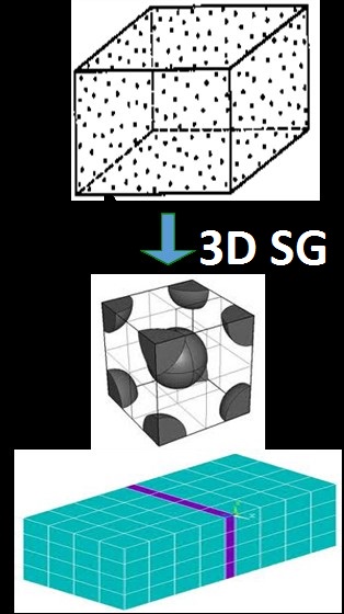
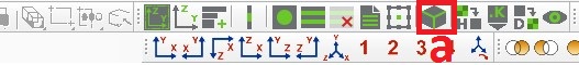
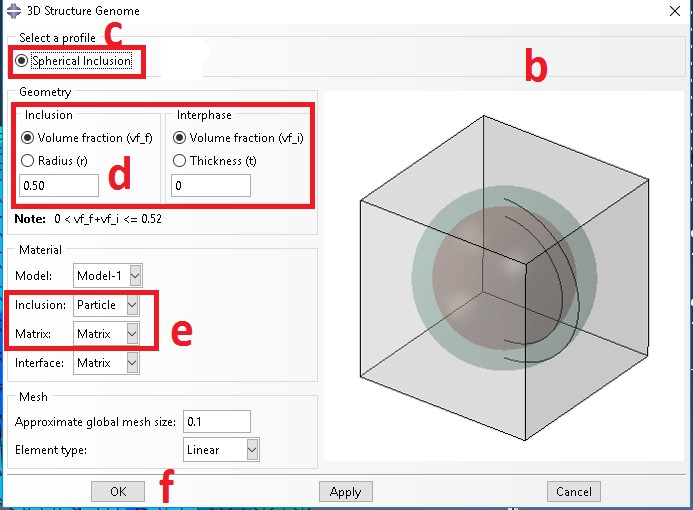
Step 2: Select appropriate SG

a. Select 3D SG that represent the current example

b. 3D SG wizard shows up
c. Select spherical inclusion as microstructure
d. Add inclusion volume fraction
e. Select material properties for inclusion and matrix
f. Click on OK to generate the SG
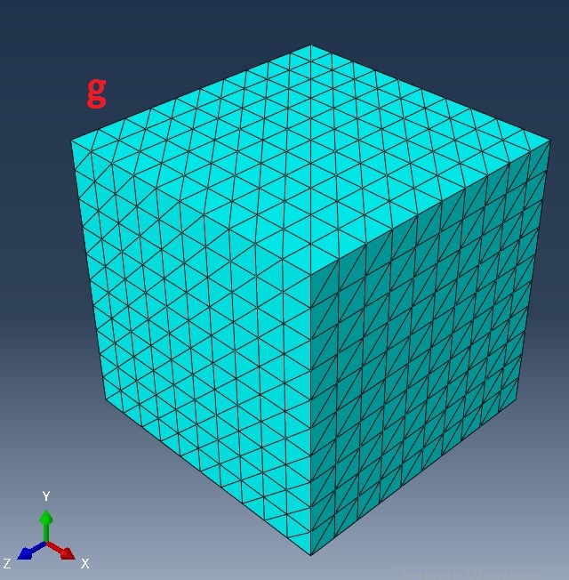
g. See generated 2D SG

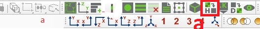
Step 3- Homogenization- 3D effective properties
a. Click on Homogenization

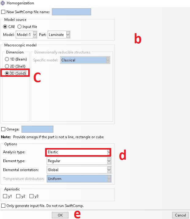
b. Homogenization wizard shows up ( see below)
c. Select 3D (solid) Model
d. Select analysis type, elastic
e. Click on OK to start homogenization
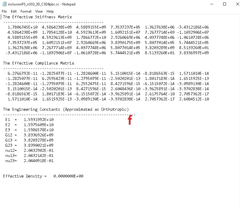
f. See the predicted 3D effective properties

Step 4: Perform dehomogenization

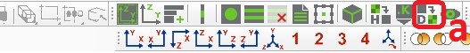
a. Select dehomogenzation

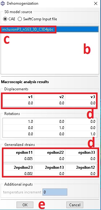
b. Dehomogenization wizard shows up
c. Select opt file
d. Add displacement to recovery displacement or strain loading to recover both local strain and stress, for current example problem let e₁₁ be 0.005 and 2e₂₃ be 0.002 e. Click on OK to start dehomogenization
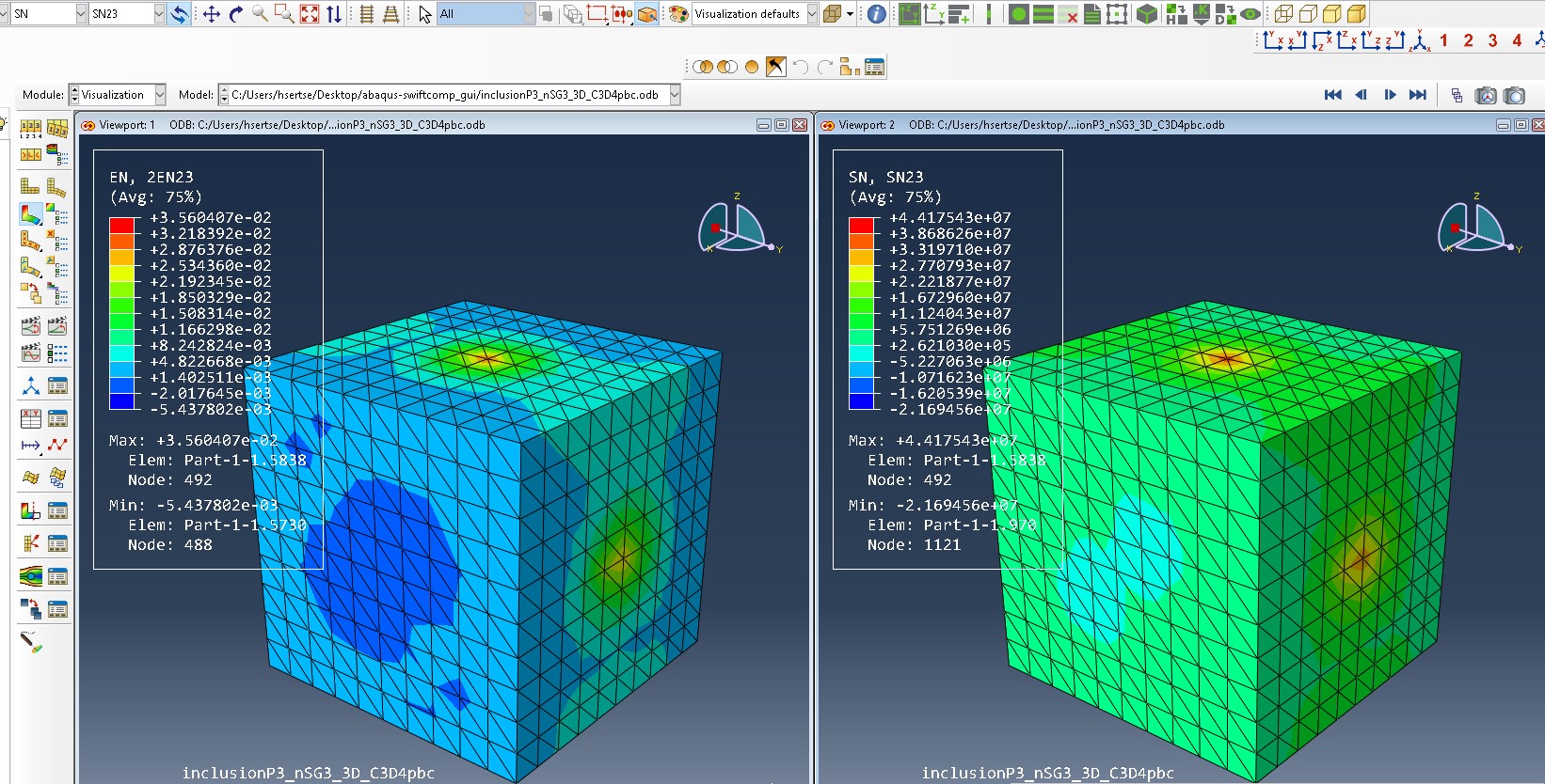
f. See, dehomogenization

youtube link:
https://youtu.be/XdmrqaI3wtw

Created on 23 Jul 2018, Last modified on 24 Jul 2018