Viscoelastic Plate Properties of a Corrugated Sandwich Sheet
In this example, we want to compute the Viscoelastic effective properties of a Corrugated Sandwich Sheet fabricated from plain weave composite material made of isotropic viscoelastic matrix and transversely isotropic elastic fiber. The MSG solid model is used to predict the effective viscoelastic properties of a plain weave composite using a three part approach.
The first part predicts the effective viscoelastic yarn properties based on the elastic fiber and viscoelastic matrix properties at the microscale. The second part takes the effective yarn properties and matrix properties to predict the viscoelastic properties of weave composites. The third part takes the effective weave properties to predict the viscoelastic properties of the Corrugated Sandwich Sheet.
 Yarn
Yarn
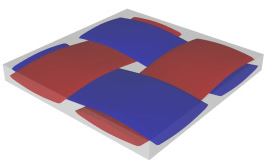 Weave
Weave
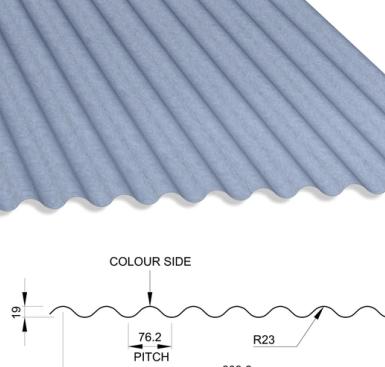 Corrugated Sheet model
 Corrugated Sandwich Sheet example
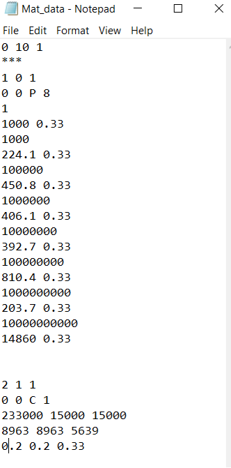
The fiber properties are defined as transversely isotropic elastic by means of engineering constants and the matrix properties are given by means of the Prony coefficients with a constant Poisson’s ratio equal to 0.33 as specified in the table below.
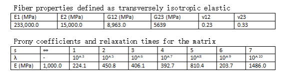 Material Properties
We will use a square pack 2D SG with fiber volume fraction equal to vf = 0.64.
Software Used
We will use TexGen4SC 2.0, SwiftComp 2.1 and Abaqus CAE with the Abaqus SwiftComp GUI for this tutorial. TexGen4SC 2.0 will be used to run the viscoelastic homogenization of the fiber-matrix square pack micro structure and also for the viscoelastic homogenization of the plain weave laminate. Abaqus CAE will be used to model the sheet and to run the viscoelastic homogenization while SwiftComp runs in the background.
Solution Procedure
The problem is solved in the following three steps:
Part 1- Micro-scale analysis of the square-pack fiber matrix micro structure using Texgen4SC.
Part 2- Meso-scale analysis of the plain weave laminate using Texgen4SC.
Part 3- Macro-scale analysis of the Corrugated Sandwich Sheet using Abaqus CAE with the Abaqus SwiftComp GUI and SwiftComp 2.1.
Part 1- Micro-scale analysis of the square-pack fiber matrix micro structure using Texgen4SC.
TexGen4SC 2.0 provides a function to let users import the material properties from a text file. Refer to the Predict viscoelastic plate properties of a single-layer plain weave laminate tutorials for more details regarding preparation of the materials text file.
Follow the step-by-step procedure to solve the problem.
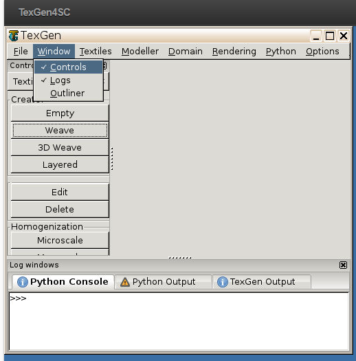
# Step 1.1. Create the plain weave pattern using TexGen4SC 2.0. Launch TexGen4SC 2.0 on cdmHUB, then Go to window-> controls-> “Weave” to create mesoscale plain weave SG.
 Weave Wizard
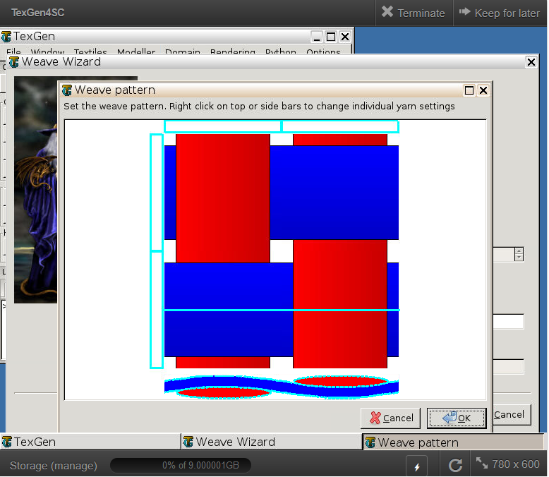
# Step 1.2. Keeping the geometric properties as required, Click on the upper-right and lower-left squares to get the woven pattern.
 Weave Pattern
# Step 1.3.Upload the .txt file containing matrix and fiber properties to the current session, using any FTP app, for example, FileZilla, to set up connection with the current session. Refer to thePredict viscoelastic plate properties of a single-layer plain weave laminate Tutorials for more details.
 Importing Material properties text file
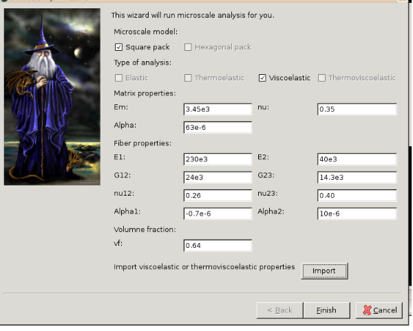
# Step 1.4. Once you uploaded the .txt file, click “Microscale” under “Homogenization” tab for yarn property calculation. Select “Viscoelastic” as the type of analysis. Set fiber volume fraction to 0.64.
 Homogenization
# Step 1.5. Ignore the matrix and fiber properties in the window, since the material properties will be imported from the uploaded file.
 Property file
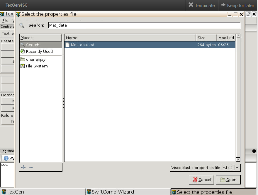
# Step 1.5. Click “Import” and select the uploaded .txt file and Click “Finish”. Now a .sc file (micro.sc) will be generated that SwiftComp will take as the input. SwiftComp will run on the cloud to calculate viscoelastic properties of yarns, e.g., effective microscale properties. In the pop-up window, you will find the analysis results.
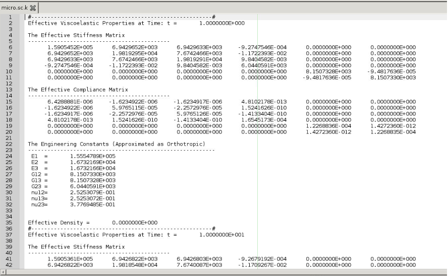 Micro scaleResuts
Part 2- Meso-scale analysis of the plain weave laminate using Texgen4SC.
# Step 2.1. Go to “File->Export->SwiftComp File” to generate the .sc file for mesoscale analysis.
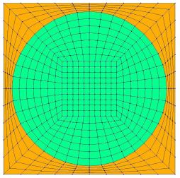
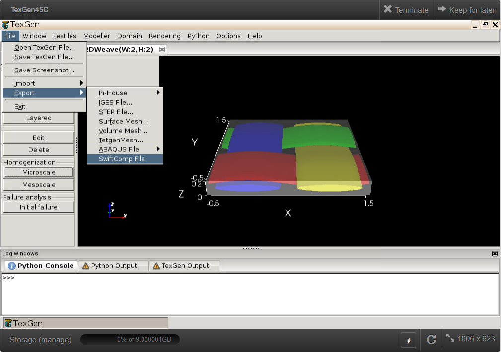 weave mesh
# Step 2.2. Define the voxel mesh, Select “Viscoelastic” as Type of analysis and Select “Plate/Shell model” and “Kirchhoff-Love plate”. Click “Select file” and select “prop_meso.txt” which is automatically generated during microscale analysis, and will be used as part of mesoscale analysis input file.
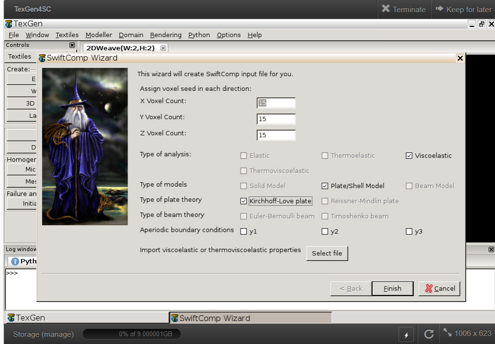 SwiftComp Wizard
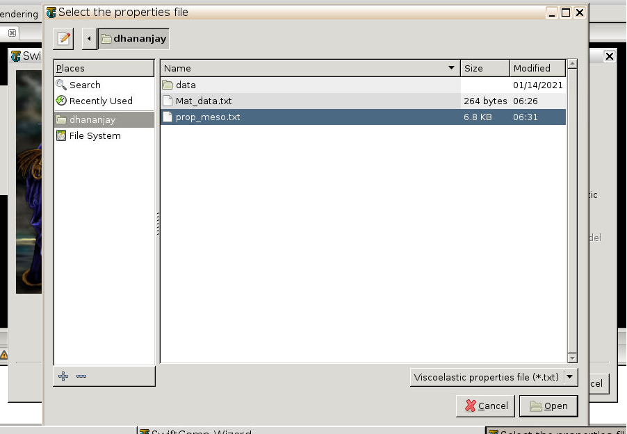 Property file
# Step 2.3. Save the .sc (SwiftComp input file) file with a filename of your choice. Click “Mesoscale” in “Homogenization” tab, which will call SwiftComp to calculate fabric properties.
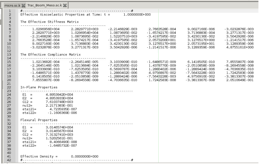 Meso Scale Results
# Step 2.4.Transfer this file to your local computer for further analysis.
Part 3- Macro-scale analysis of the Corrugated Sandwich Sheet using Abaqus CAE with the Abaqus SwiftComp GUI and SwiftComp 2.1.
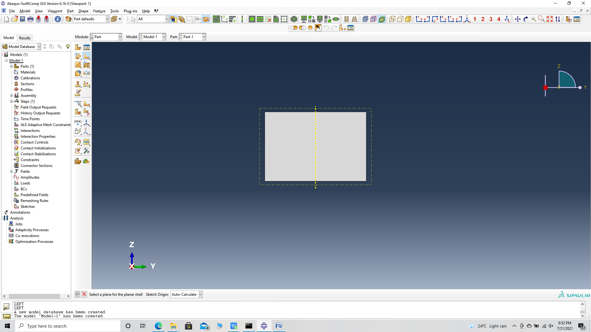
# Step 3.1. Using Abaqus CAE with the Abaqus SwiftComp GUI plugin, Create the part geometry for the Corrugated Sandwich Sheet. Use Set sketch plane for customized SG -> Create planar shell -> Select the plane and vertical axis -> Sketch the rectangle shown and create the part.
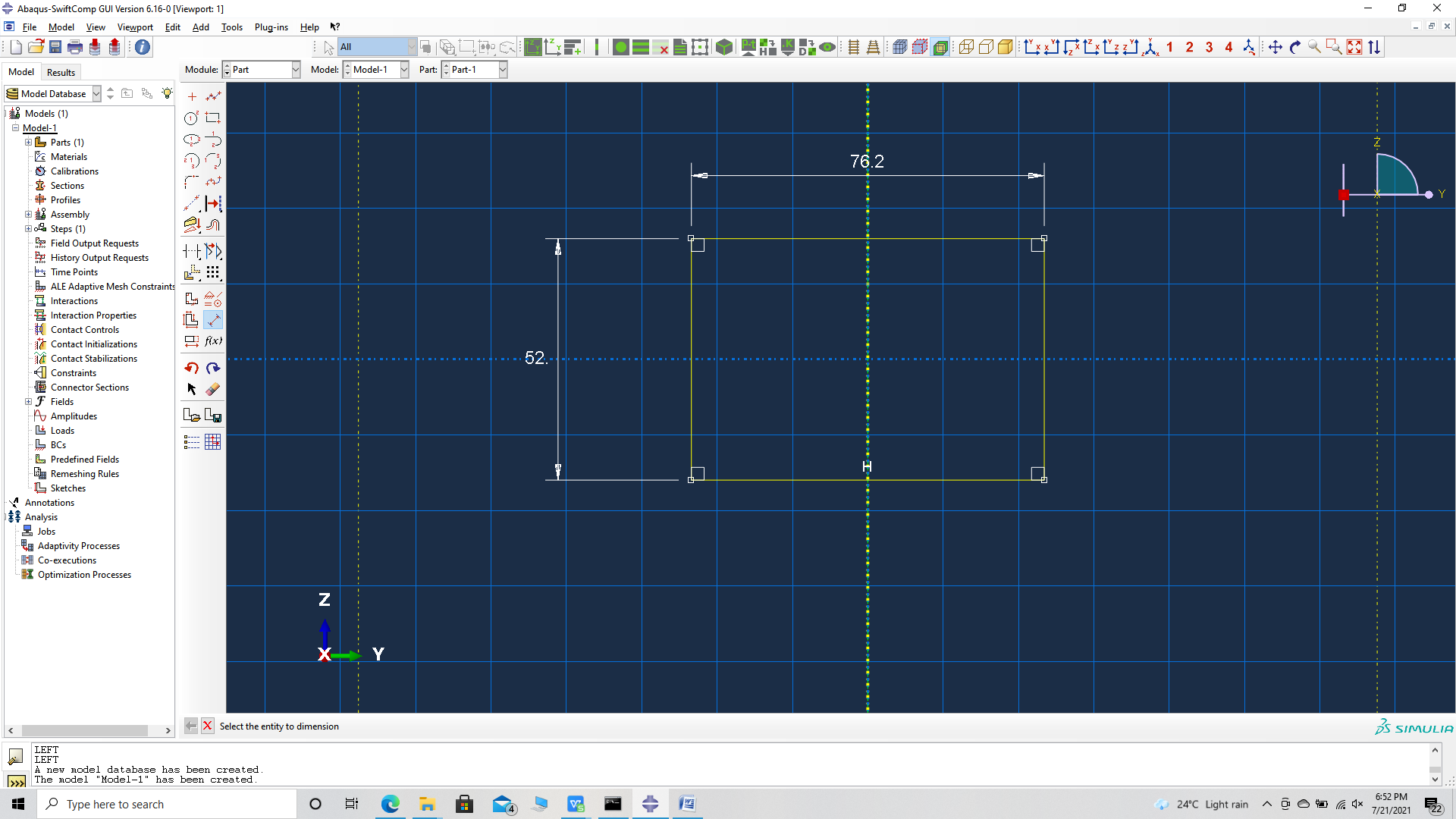 Part Geometry
 Part Geometry
# Step 3.2. Partition the part as shown to obtain the required cross-section. We focus on one quadrant and later mirror our partition lines to the other quadrants. Firstly add two horizontal partition lines, three horizontal construction lines, one vertical partition line and one vertical construction line as shown.
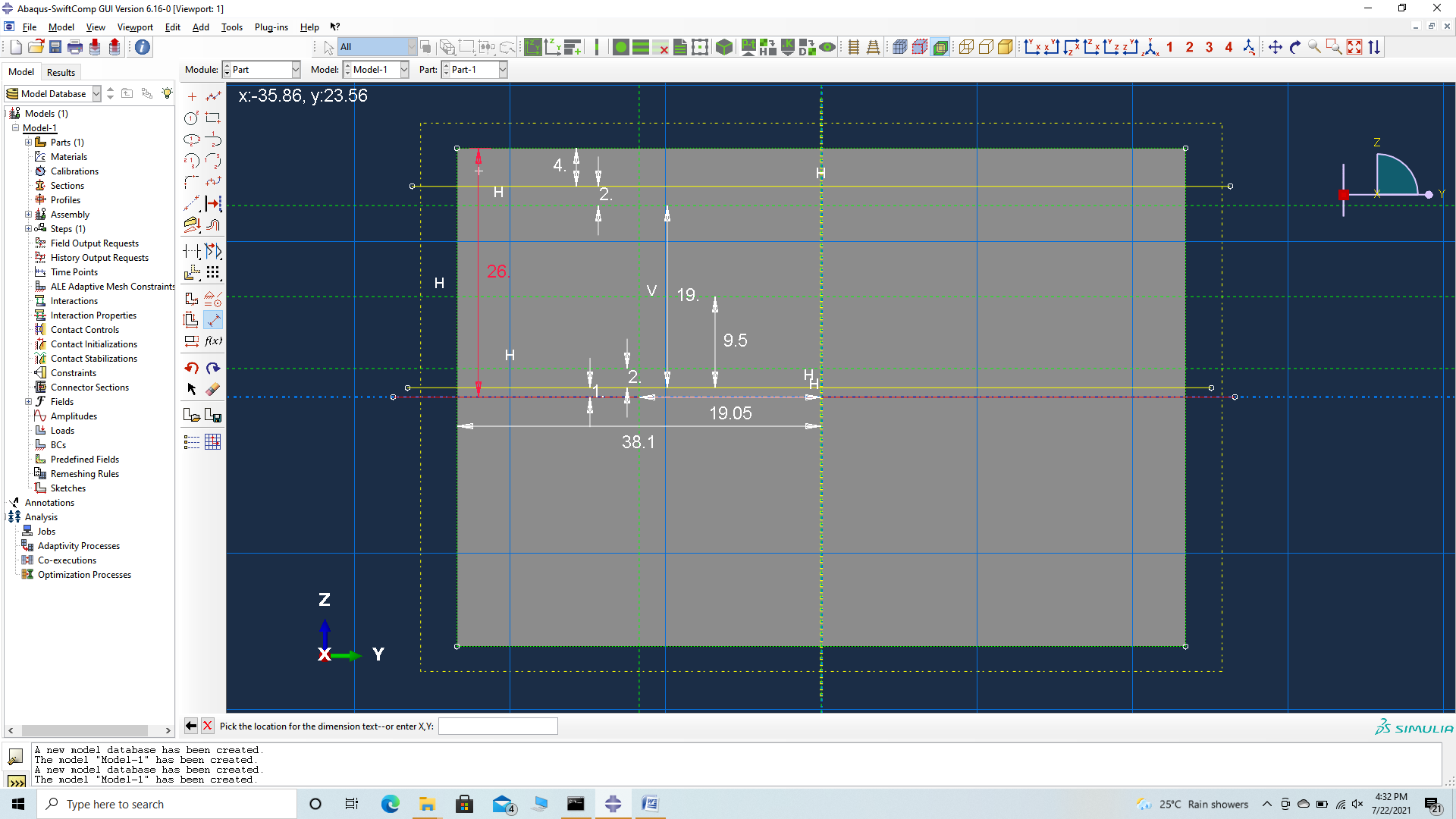 first set of Partitions
# Step 3.3. Now add two arcs using create arc tru three points as shown. Fix their starting points on the vertical partition, and choose their end points on the second horizontal construction line and choose their third point at random. Constrain their concentricity and set the inner radius as 23 mm. Add partitions to the curves to help add their material properties later.
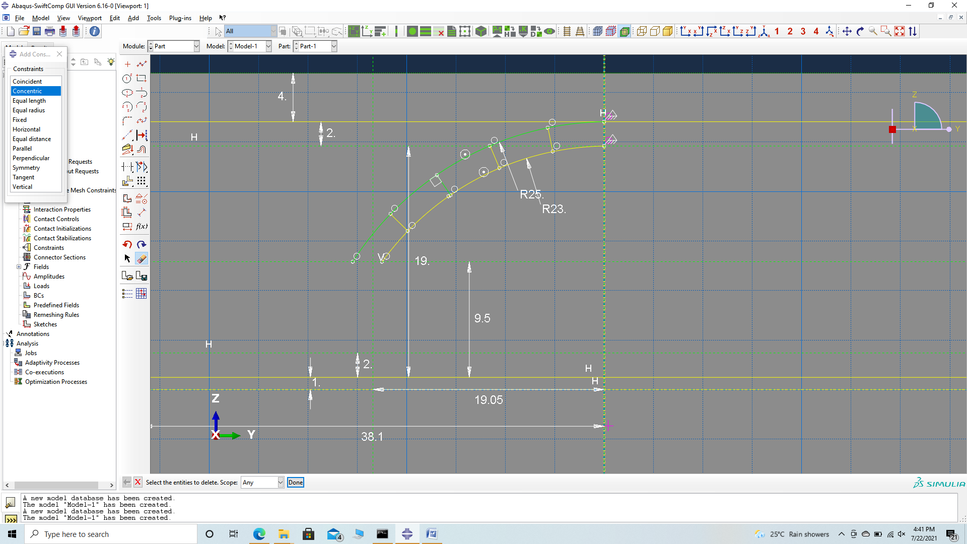 second set of Partitions
# Step 3.4. Now add the other two arcs of the quadrant as shown. Fix their starting points on the edge, and choose their end points on the second horizontal construction line coinciding with the ends of the previous arcs and choose their third point at random. Constrain their concentricity. Add partitions to the curves to help add their material properties later. Now adjust the meeting of the two pairs of curves to smooth en it by, trimming the sections they meet and replacing it with a new pair of curves which is sectioned so that the section line passes through the intersection of the second horizontal construction line and the vertical construction line as shown.
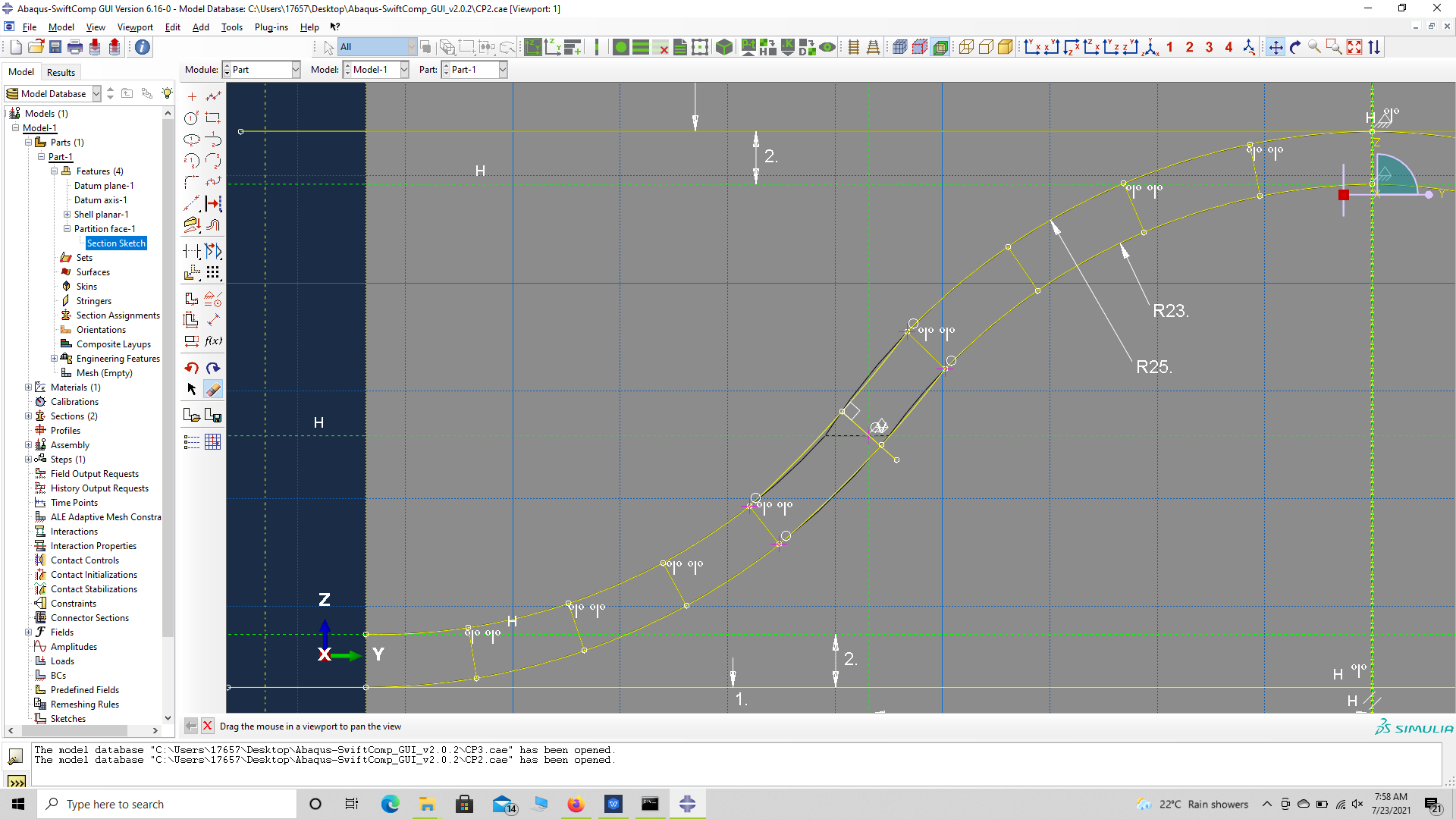 Third set of Partitions
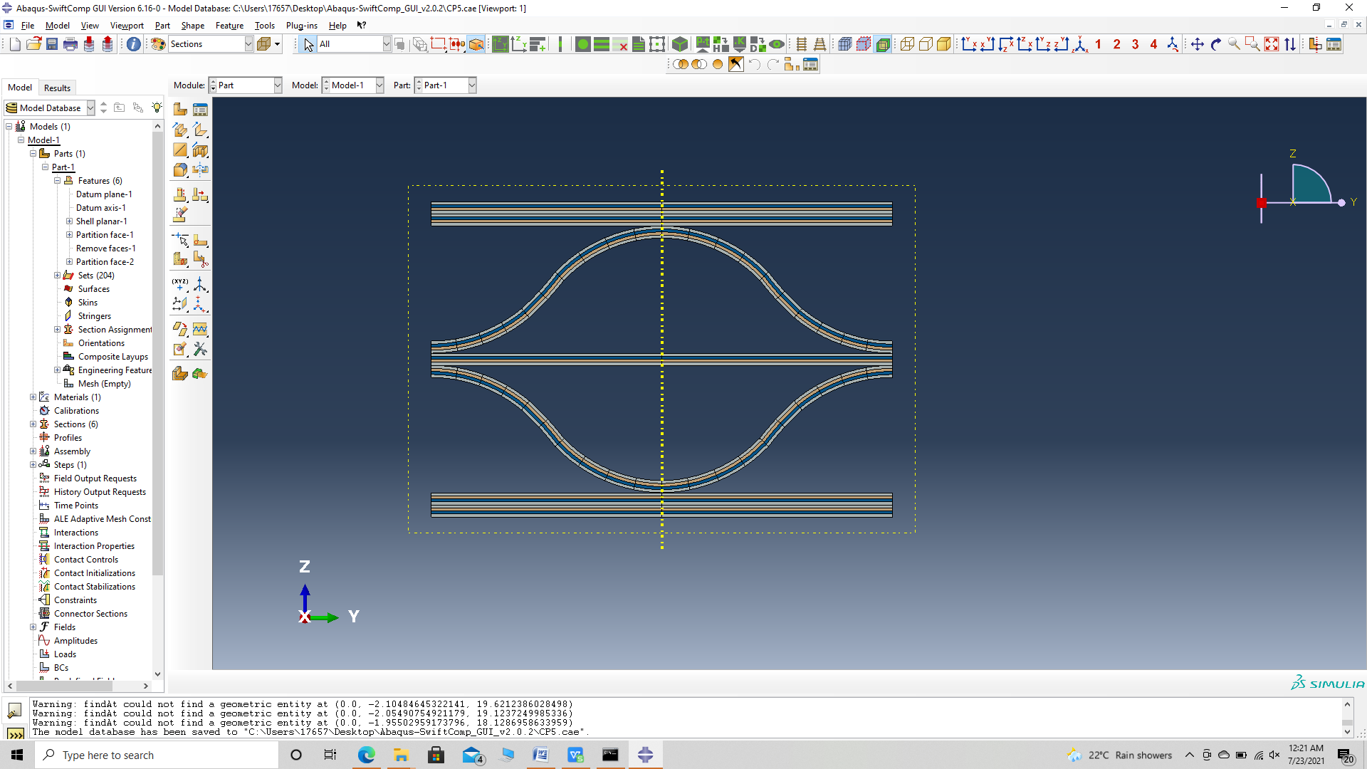
# Step 3.5. Mirror the partition lines for the other quadrants to have the partition lines shown.
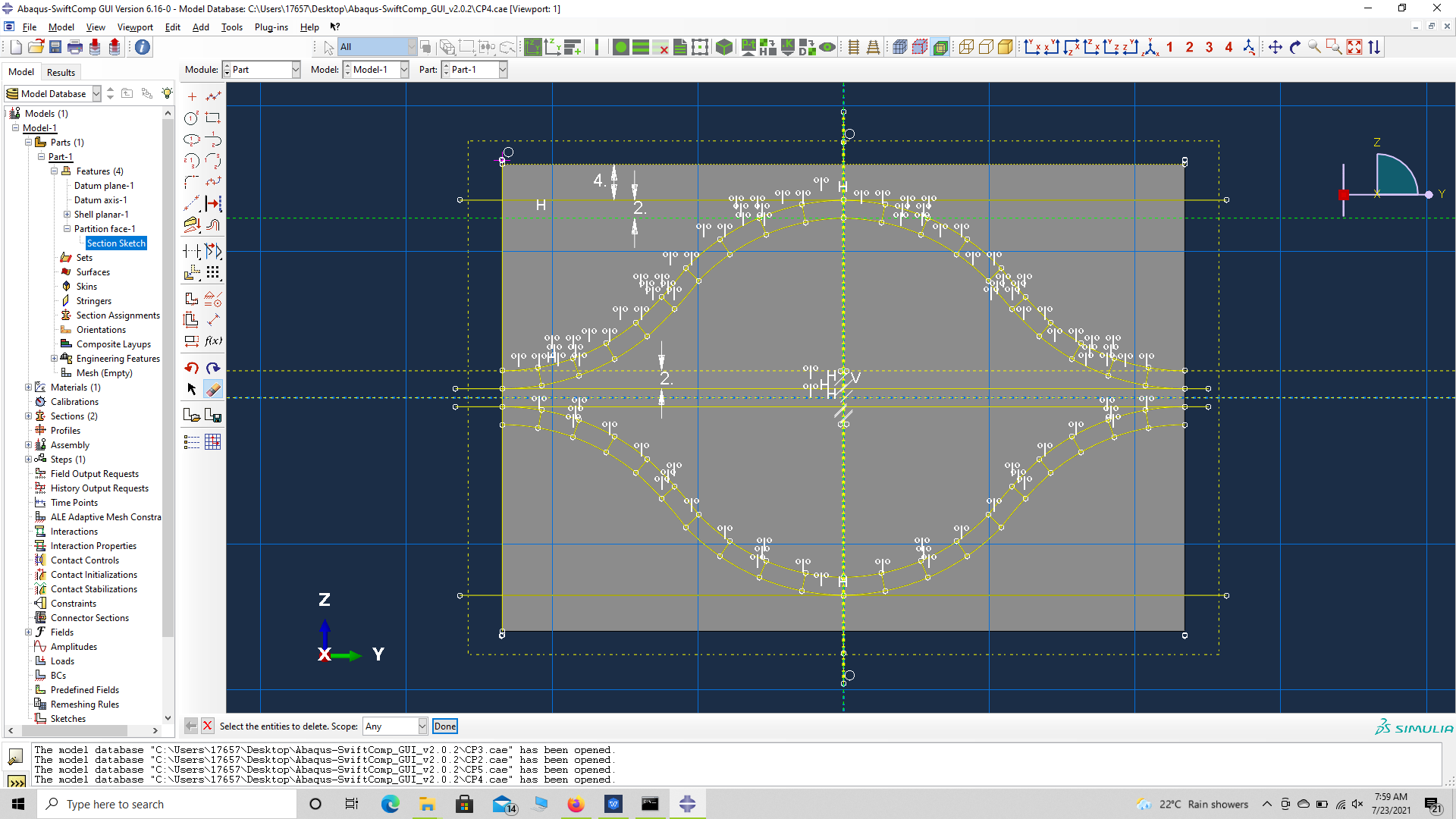 Fourth set of Partitions
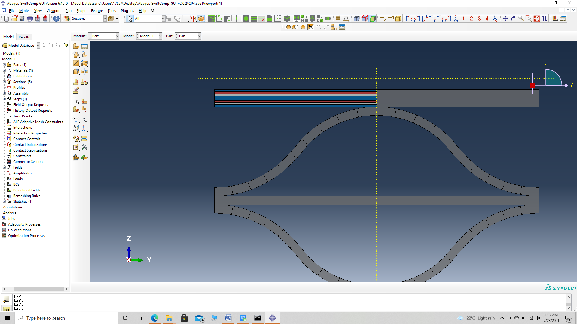
# Step 3.6. Create the part and delete the redundant faces to have the final part shown.
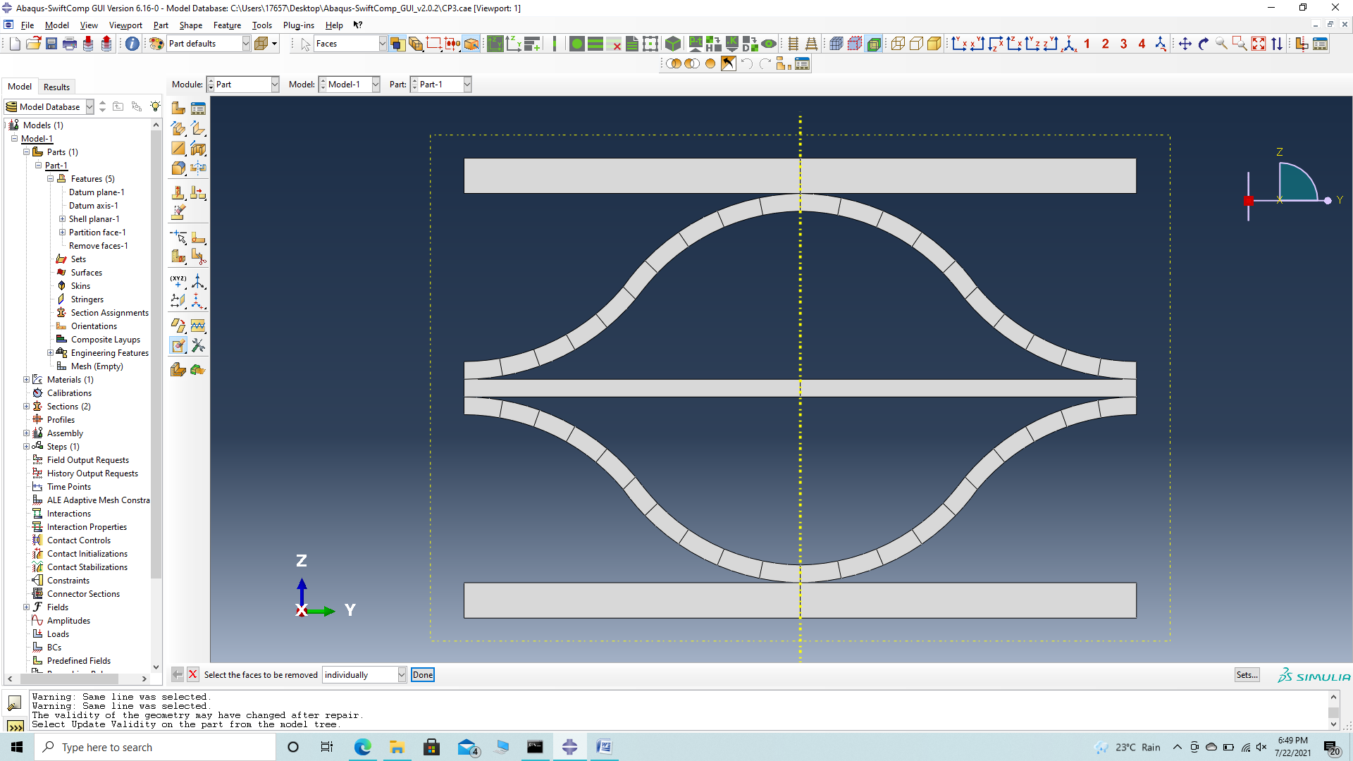 Sandwich corrugated sheet
# Step 3.7. To enter the material properties for the part, first we need to choose the material properties from the results of the computed effective viscoelastic properties in the previous part. Within the Materials section of Abaqus CAE, we create a dummy material called “Material”. Please note that we will not define the material properties using the Abaqus SwiftComp GUI. refer to the Computation of effective viscoelastic properties with Abaqus SwiftComp GUI tutorial for more details.
 dd
dd
# Step 3.8.Import the material properties from the previous step. Since the material properties are given as a time-dependent properties, We will create a text file to input the time-dependent material properties described row wise as –
We will use the in plane engineering constants defined by means of engineering constants unless If we are modelling for flexure, we will use the flexural properties. We will define the material properties in the text file as
Orthotropic defined by means of engineering constants. —- E1 (t) —- E2 (t) —- E3 (t) —- nu12 (t) —- nu13 (t) —- nu23 (t) —- G12 (t) —- G13 (t) —- G23 (t) —- Time, t for all time intervals.
(Image(CS3.81.png, desc="Material properties file") failed - File not found)
# Step 3.9. Now go to New Layups and add the material, section name, Layup and thickness to create the required layup. This can be repeated if we have multiple layups. We will use (0/45/-45/0)2 and (0/45/-45/0) as the laminate for the sheet.
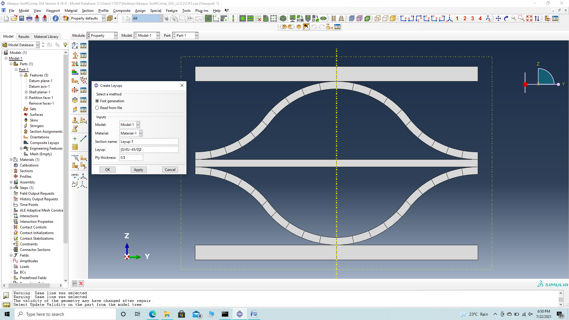 First Layup
 Second Layup
‘ # Step 3.10. To assign the layup, go to Create 2D SG: Assign Layups and the pick the baseline, the line opposite to the baseline and the area between the two picked line for the right flange as shown and then hit Ok. Do this for all sections
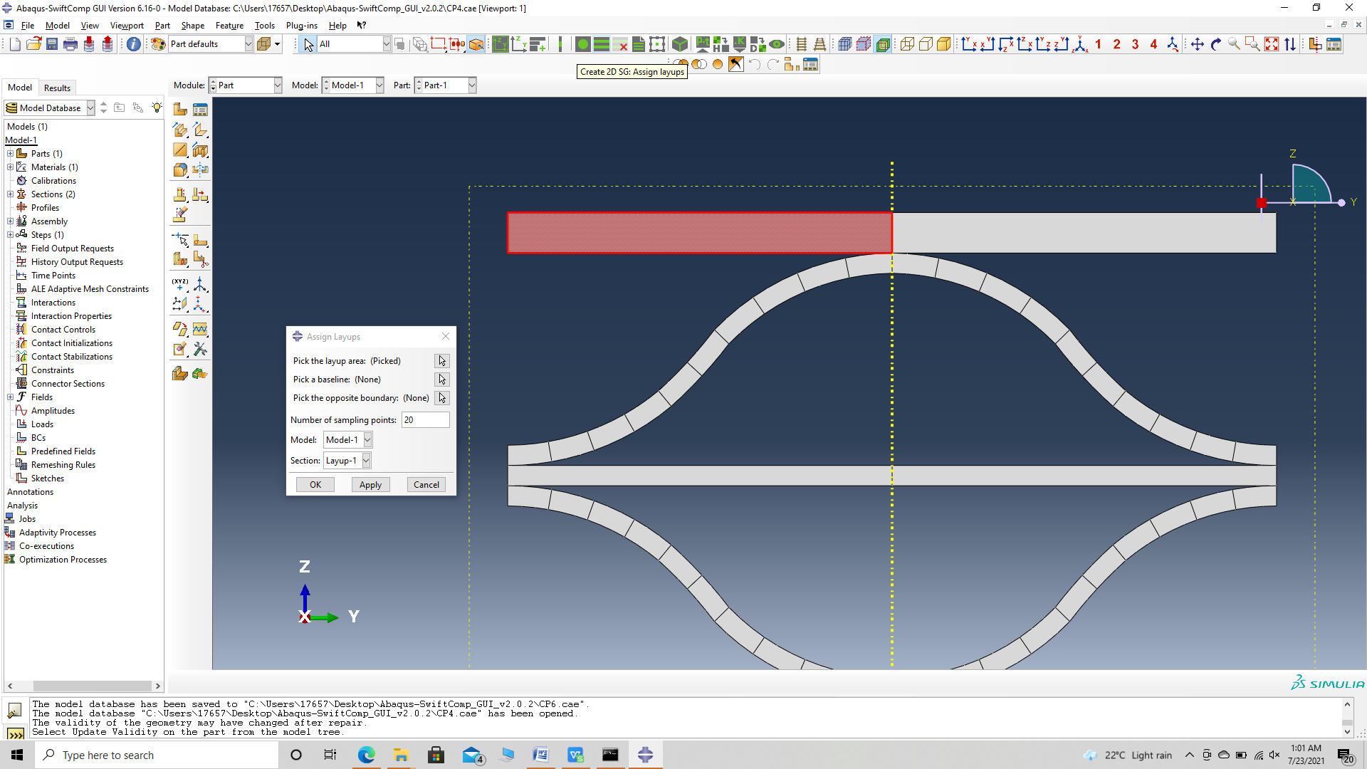 Layp area
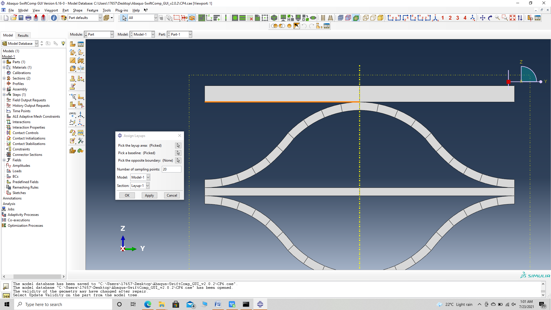 Baseline
 opposite edge
 Assigned Layup
 Assigned Layups
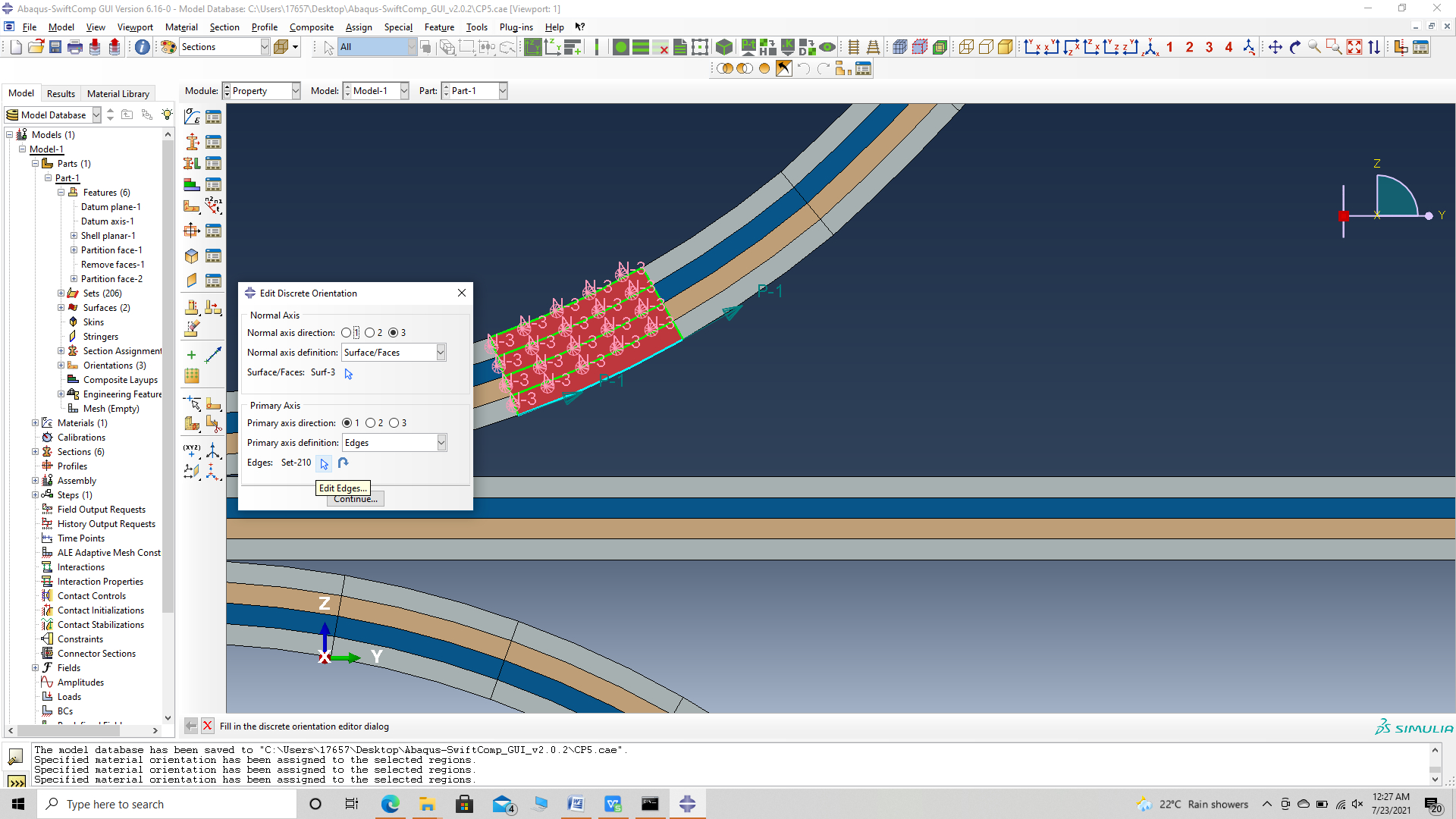
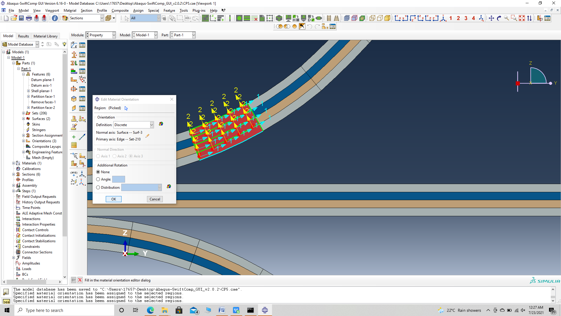
‘ # Step 3.11. Now we assign the material orientation for the part. Go to Assign material orientation -> select the sections of the partto be assigned orientation -> Done -> Select a CSYS (use default orientation or other method) -> Definition (Discrete) -> Define -> Primary axis orientation -> choose edge and flip direction if needed to make the axis point towards the layp direction direction -> Choose the surfaces for the normal axis definition -> Continue -> OK. Orientation Axis 1 represents the y2 axis of SwiftComp’s local orientation and orientation axis 2 represents y3 axis of SwiftComp’s local orientation. Now go to Assemble, create the part instance with dependent mesh.
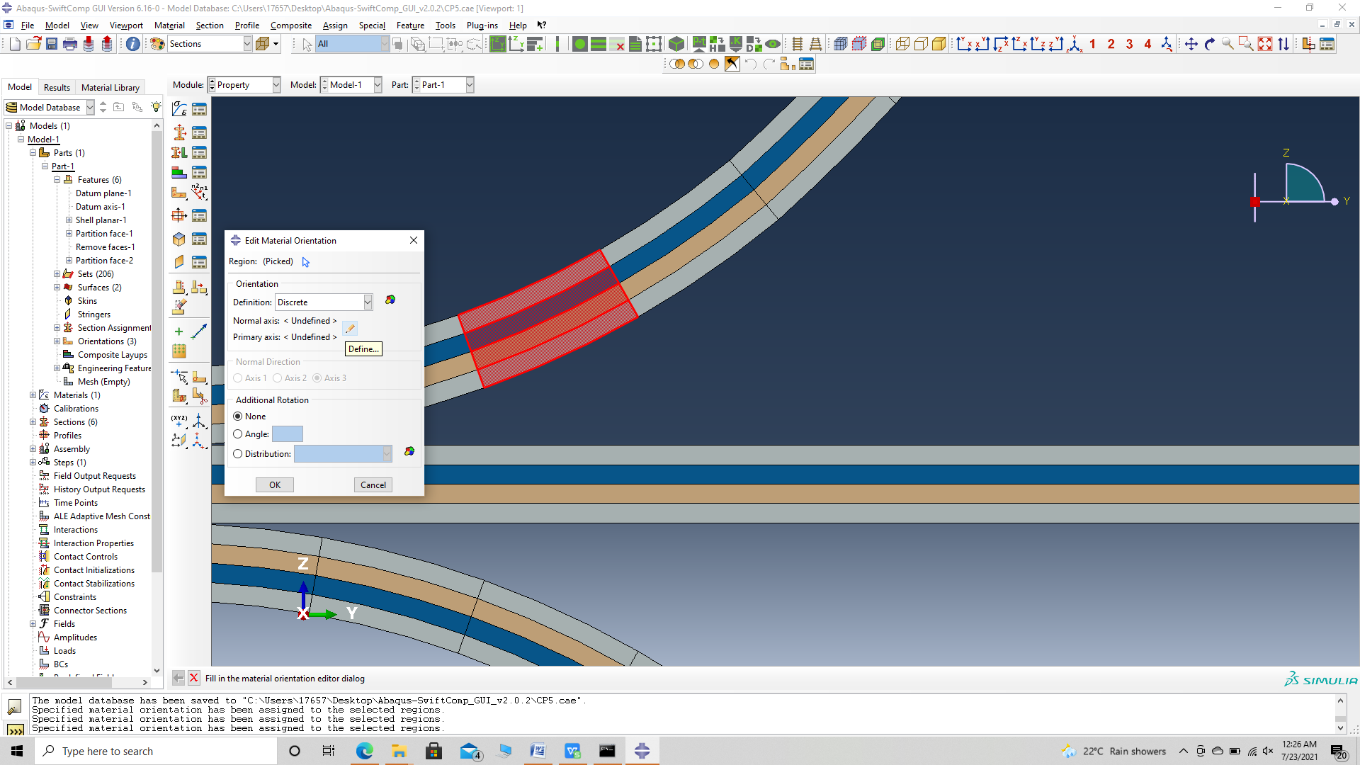 Assign material orientation
 Define orientation
 Orientation
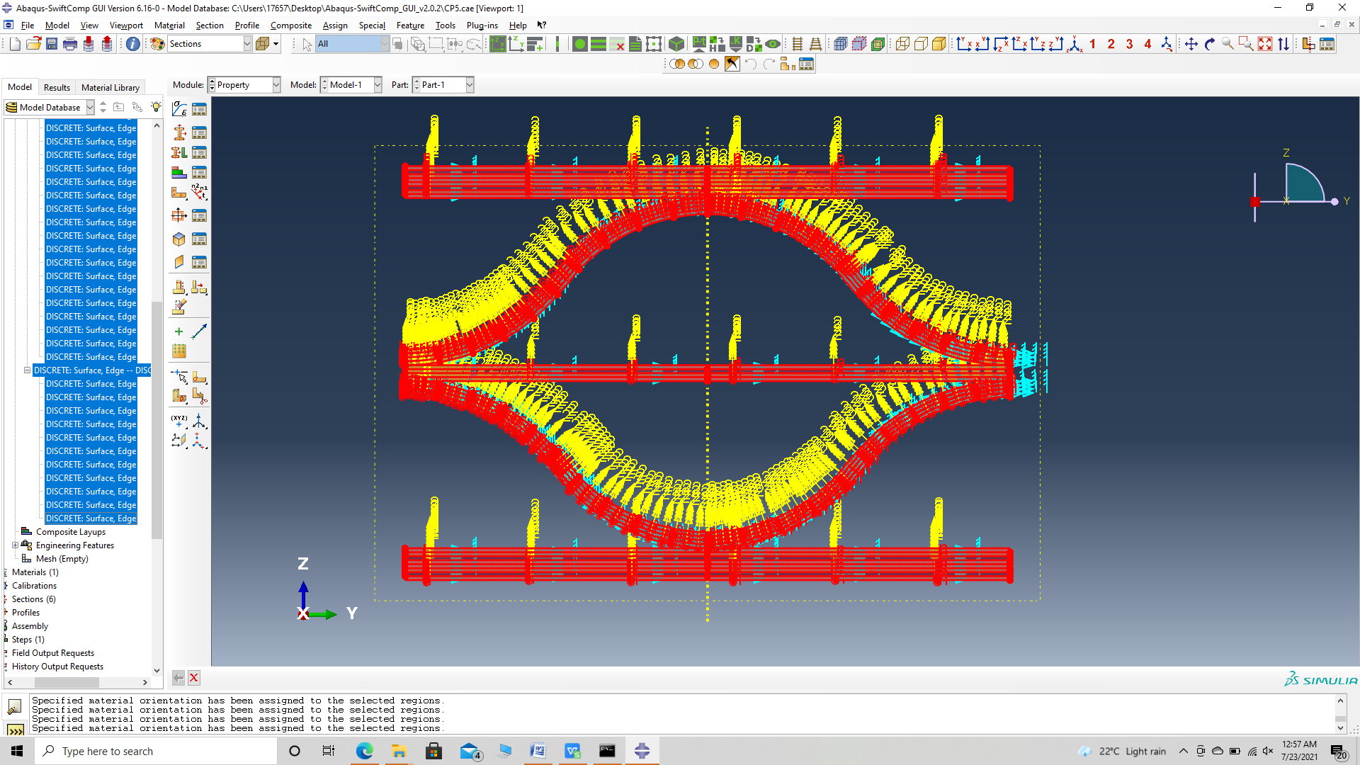 Part Orientation
‘ # Step 3.12. Now go to Assemble, create the part instance with dependent mesh.
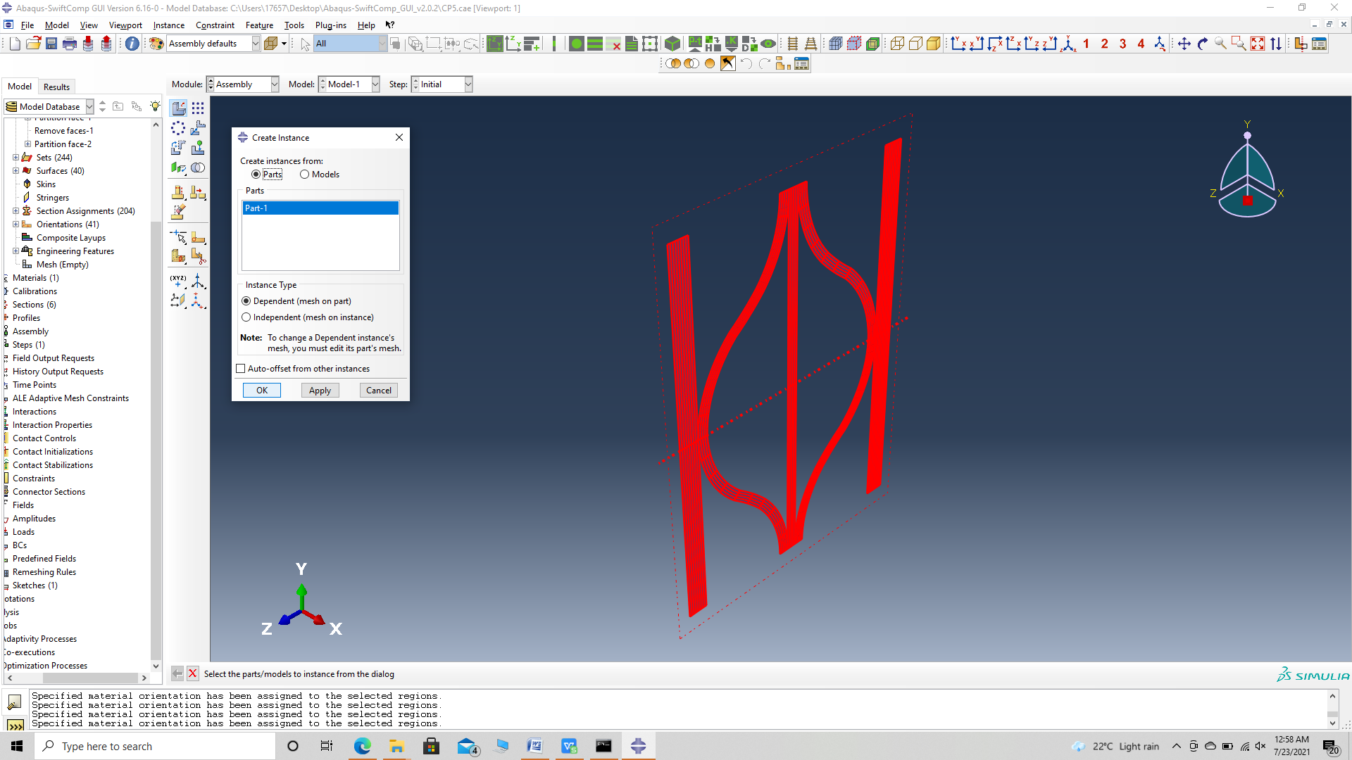 assembly
# Step 3.13.In the Mesh section, Seed the Part and set approximate global mesh size, then Click ‘Mesh Part’
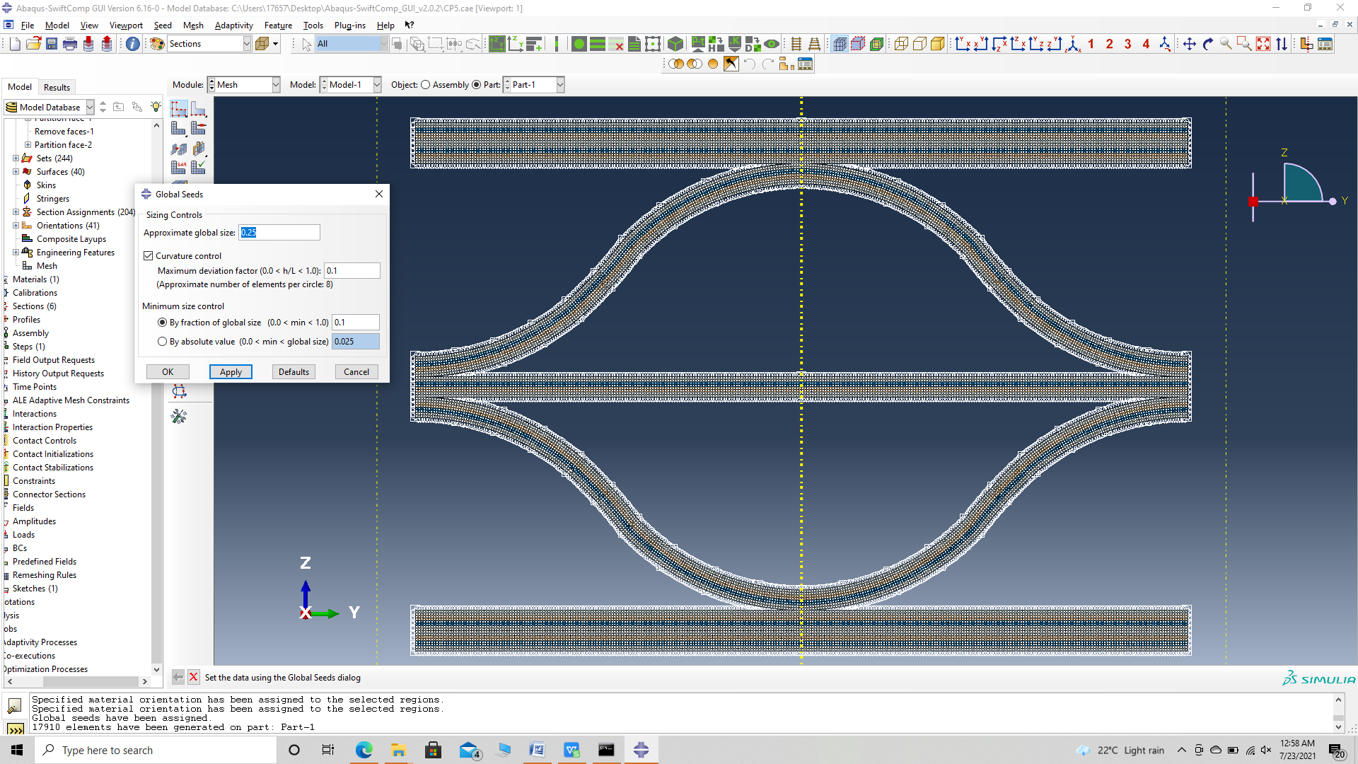 Mesh
Mesh
# Step 3.14.Create a job and write its input file.
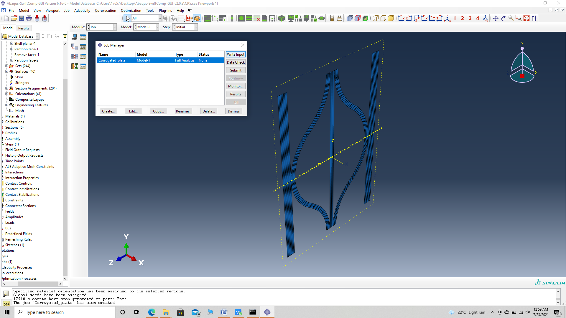 ip file
# Step 3.15. Homogenize the part preferably as a plate using the Homogenization via input file option to get the final results. In the Viscoelastic/Thermoviscoelastic Analysis section, we define the range of the time (i.e. Initial time” and Final time”) in which we want to output the effective properties as well as the frequency (i.e. Time increment” defined in decades).
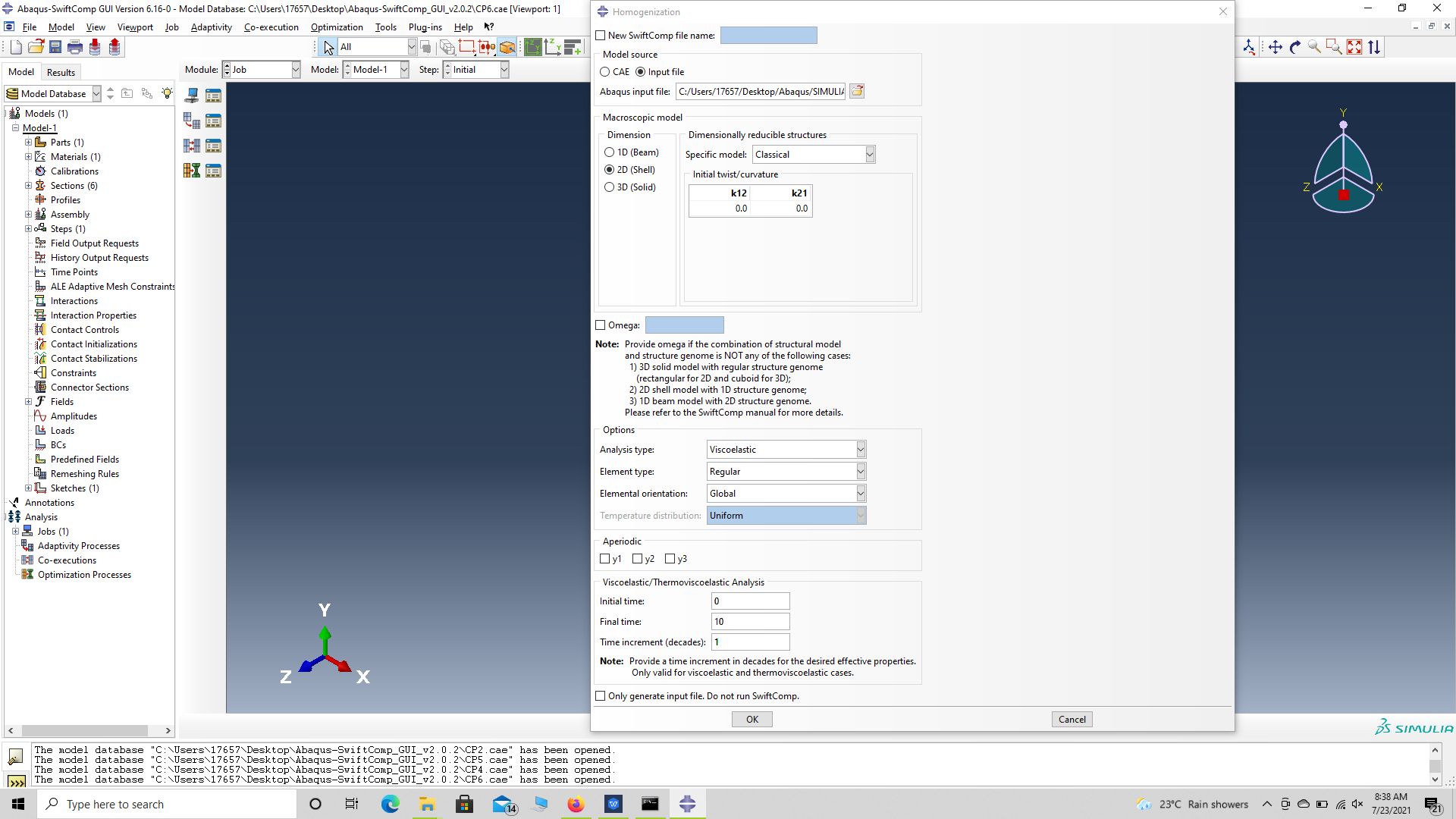 Homogenization
References
# Rique, O.; Liu, X.; Yu, W., Pipes, R. B.: “Constitutive modeling for time- and temperature-dependent behavior of composites,” Composites Part B: Engineering, Vol 184, March 2020, DOI: 10.1016/j.compositesb.2019.107726.