Elastic analysis of an Airfoil with uniform cross-section
In this example, we want to compute the elastic effective properties of an Airfoil with uniform cross-section, fabricated from plain weave lamina made of isotropic elastic matrix and transversely isotropic elastic fiber. The MSG solid model is used to predict the effective elastic properties of a plain weave composite using a three part approach. The Airfoil model is derived from H. Chen, W. Yu and M. Capellaro and the Airfoil baselines taken from UIUC Airfoil Coordinate Database, mh104 model.
The first part predicts the effective elastic yarn properties based on the elastic fiber and matrix properties at the micro-scale. The second part takes the effective yarn properties and matrix properties to predict the elastic properties of weave composites. The third part uses the effective weave properties in the 3D Macro-scale analysis to predict the elastic properties of the Airfoil .
 Yarn
Yarn
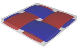 Weave
Weave
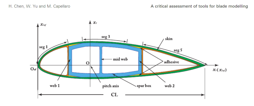 Airfoil model taken from H. Chen, W. Yu and M. Capellaro
 Airfoil baselines taken from UIUC Airfoil Coordinate Database mh104 model'
The fiber properties are defined as transversely isotropic elastic by means of engineering constants and the matrix properties are given by means of the elastic modulus with a constant Poisson’s ratio equal to 0.33 as specified in the table below.
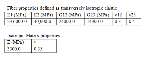 Material Properties
We will use a square pack 2D SG with fiber volume fraction equal to vf = 0.64.
Software Used
We will use TexGen4SC 2.0, SwiftComp 2.1 and Abaqus CAE with the Abaqus SwiftComp GUI for this tutorial. TexGen4SC 2.0 will be used to run the elastic homogenization of the fiber-matrix square pack microstructure and also for the elastic homogenization of the plain weave laminate. Abaqus CAE will be used to model the tube and to run the homogenization while SwiftComp runs in the background.
Solution Procedure
The problem is divided into the following five sections:
Section 1- 2D Micro-scale analysis of the square-pack fiber matrix micro structure using Texgen4SC.
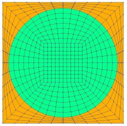
Section 2- 3D Meso-scale analysis of the plain weave laminate using Texgen4SC2.0.
Section 3- 3D Macro-scale analysis of the Airfoil using Abaqus CAE with the Abaqus SwiftComp GUI and SwiftComp 2.1.
Section1- Micro-scale analysis of the square-pack fiber matrix micro structure using Texgen4SC.
# Step 1.1. Create the plain weave pattern using TexGen4SC 2.0. Launch TexGen4SC 2.0 on cdmHUB, the Go to window-> controls-> “Weave” to create mesoscale plain weave SG.
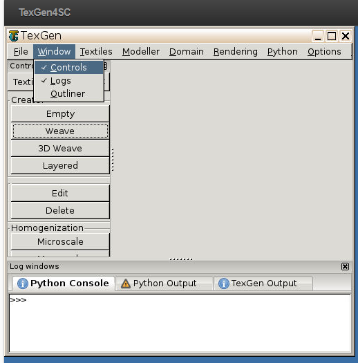 Weave Wizard
# Step 1.2. Keeping the geometric properties as required, Click on the upper-right and lower-left squares to get the woven pattern.
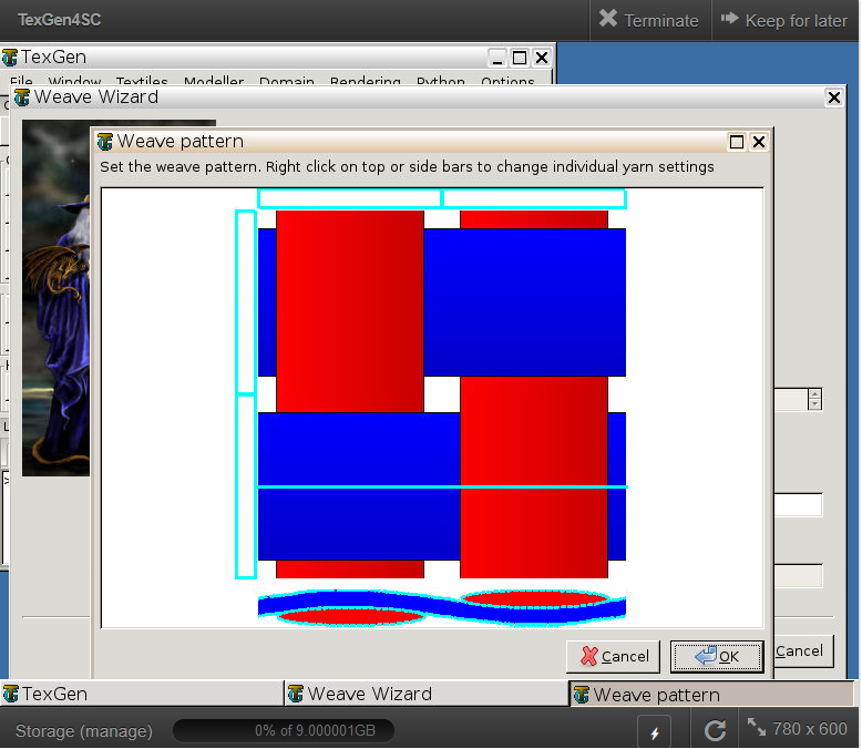 Weave Pattern
# Step 1.3.Click “Microscale” under “Homogenization” tab for yarn property calculation. Select “elastic” as the type of analysis and Enter the material properties for the fiber and matrix and set fiber Volume fraction as 0.64 and Click “Finish”.
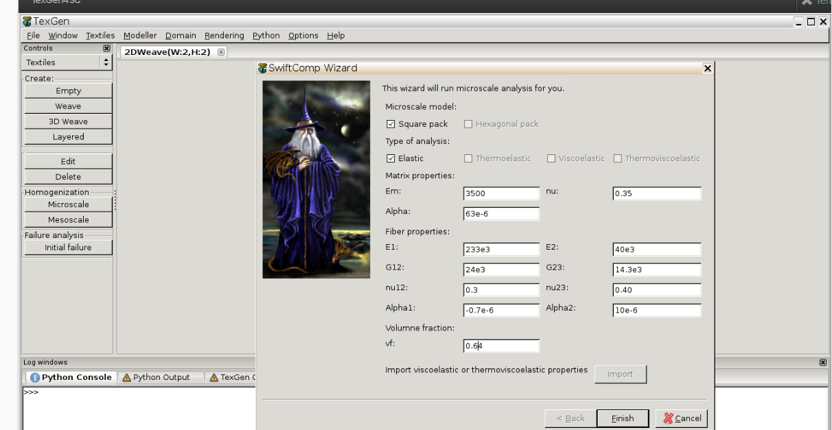 Adding Material properties
# Step 1.4. Now a .sc file (micro.sc) will be generated that SwiftComp will take as the input. SwiftComp will run on the cloud to calculate elastic properties of yarns, e.g., effective microscale properties. In the pop-up window, you will find the analysis results.
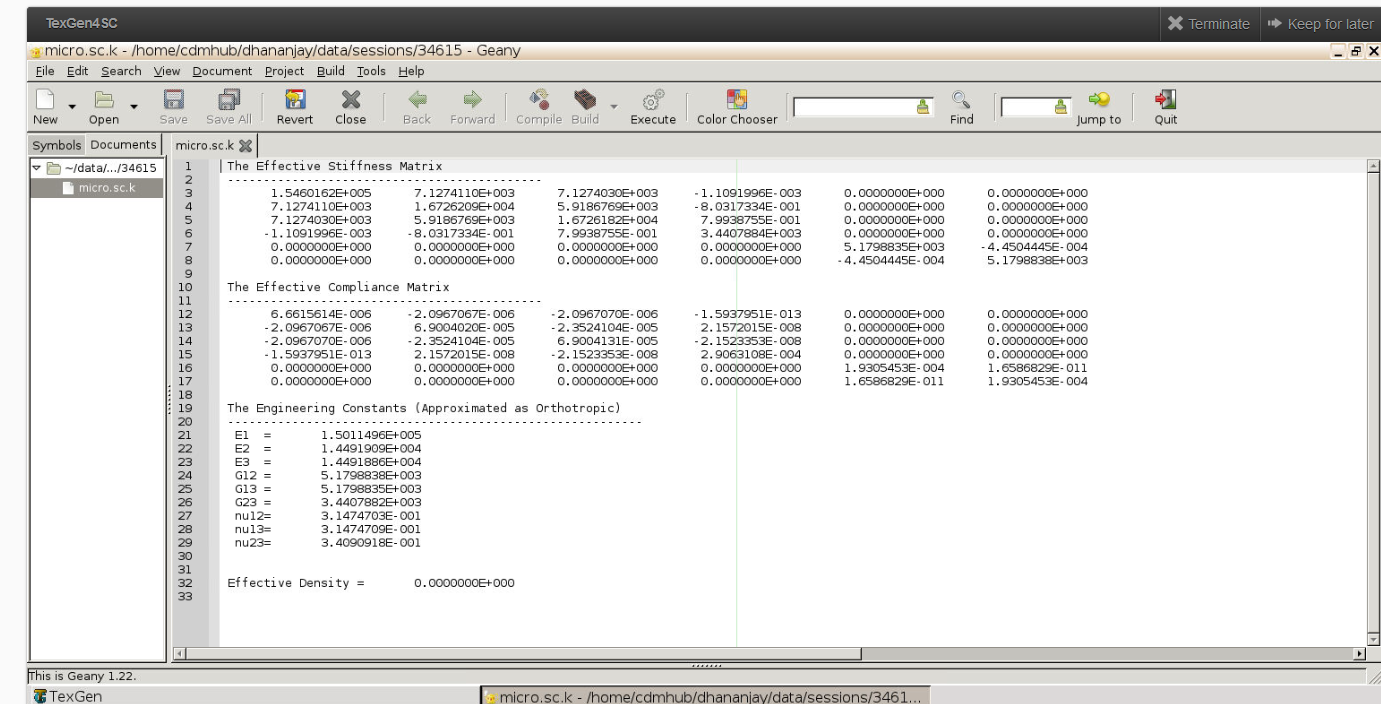 Micro scaleResuts
Section 2- Meso-scale analysis of the plain weave laminate using Texgen4SC.
# Step 2.1. Go to “File->Export->SwiftComp File” to generate the .sc file for mesoscale analysis.
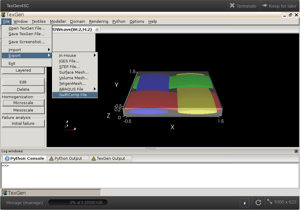 weave mesh
# Step 2.2. Define the voxel mesh, Select “elastic” as Type of analysis and Select “Solid Model”.
 SwiftComp Wizard
# Step 2.3. Save the .sc (SwiftComp input file) file with a filename of your choice. Click “Mesoscale” in “Homogenization” tab, which will call SwiftComp to calculate fabric properties.
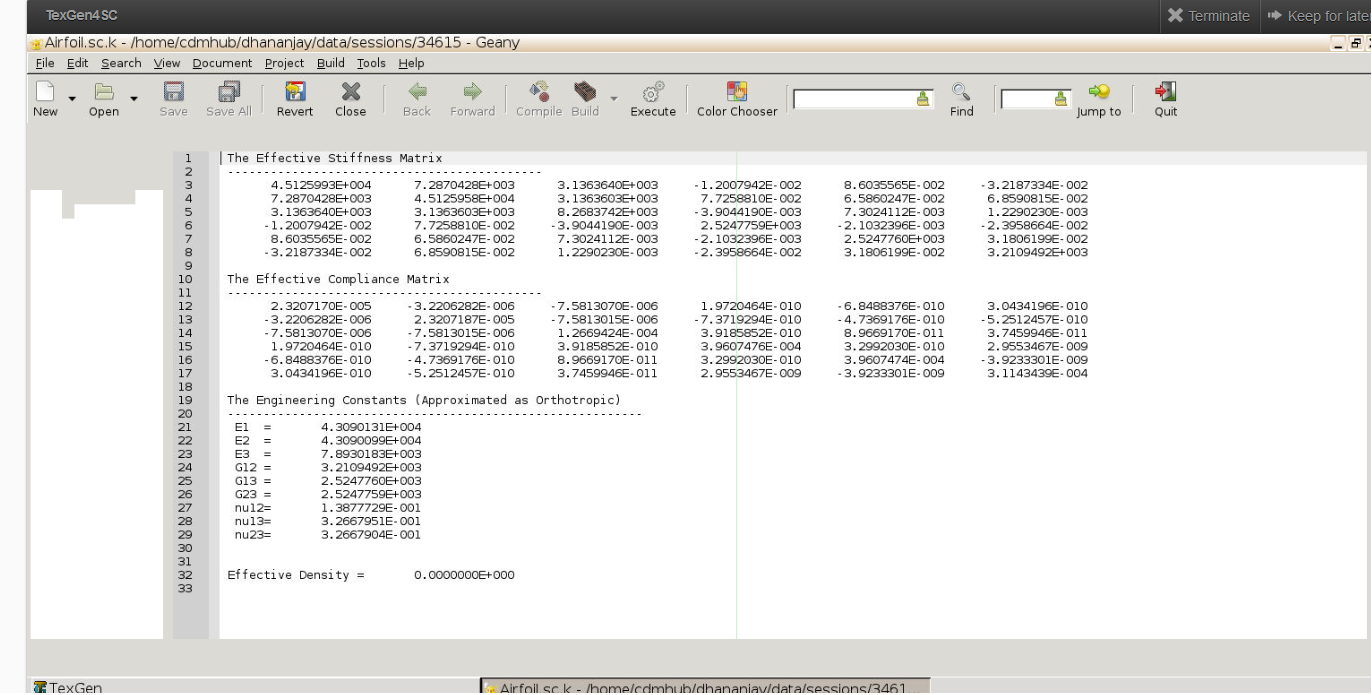 Meso Scale Results
# Step 2.4.Transfer this file to your local computer for further analysis.
Section 3- Macro-scale analysis of the Airfoil using Abaqus CAE with the Abaqus SwiftComp GUI and SwiftComp 2.1.
# Step 3.1. Set sketch plane for customized SG -> Create planar shell -> Select the plane and vertical axis -> Sketch the cross section shown from the baseline coordinates.
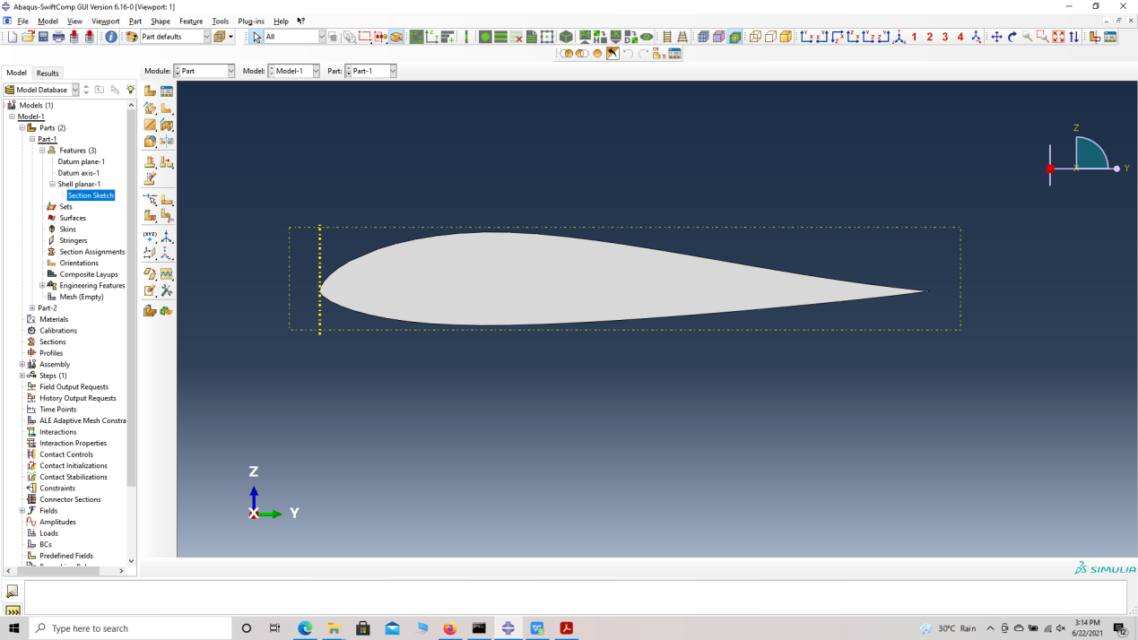 Airfoil shell
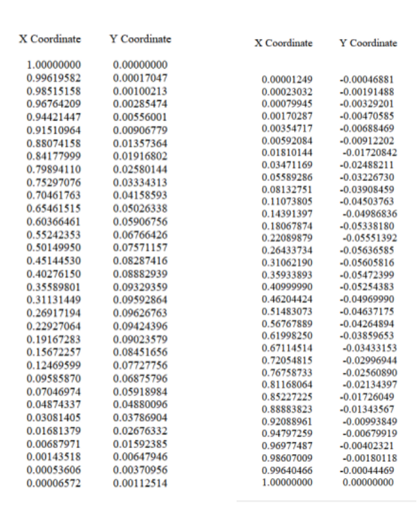 Baseline coordinates
# Step 3.2. Partition the part as shown to obtain the final cross-section
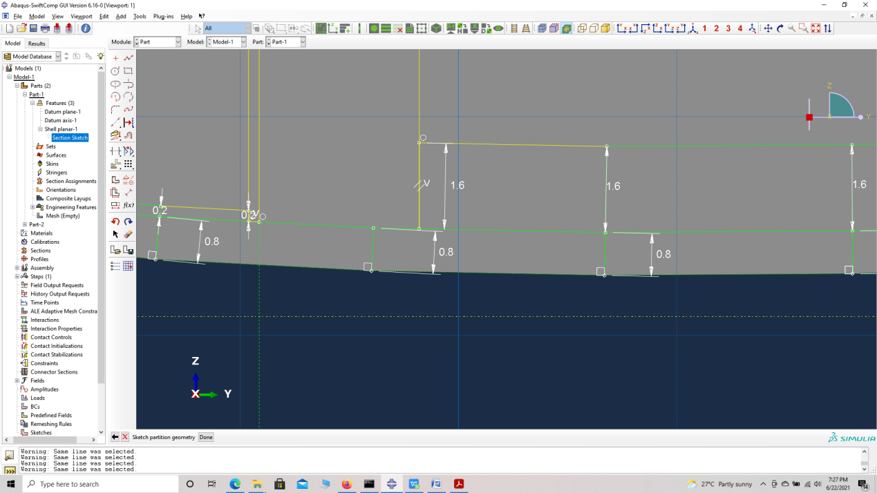 Airfoil shell partition dimensions
 Airfoil shell partition
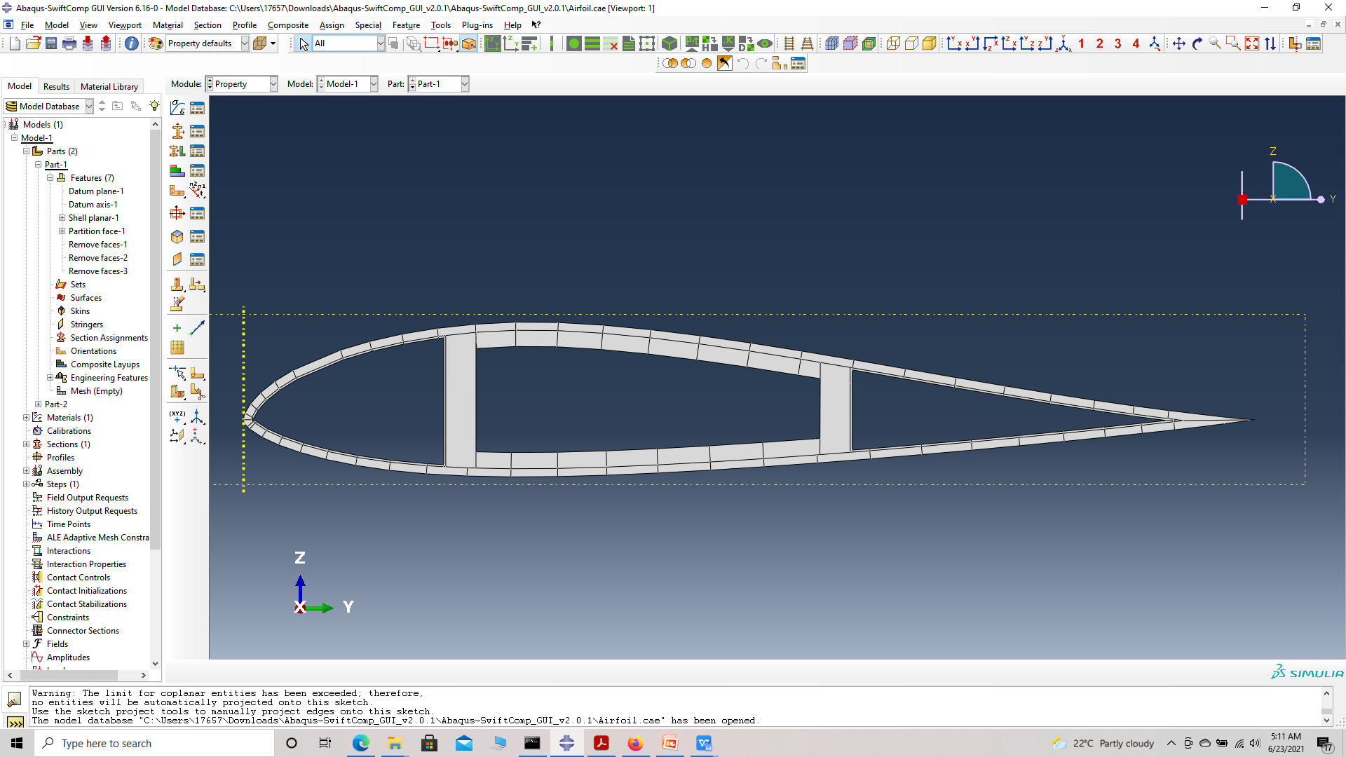 Airfoil Crosssection
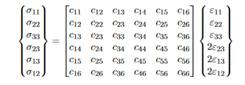
# Step 3.3. Enter the material properties for the model. First we need to choose the material properties from the results of the computed effective elastic properties in the previous part. Then we need to convert the Constitutive relations provided as SwiftComp’s results into Abaqus’s Constitutive relations. This can be done by switching the 4th and 6th rows for the relation and also switching the 4th and 6th column of the stiffness matrix. The relations are provided below. Within the Materials section of Abaqus CAE, we create a material called “Material-1” and add the corresponding properties. We can also import the homogenized properties from the toolbar.
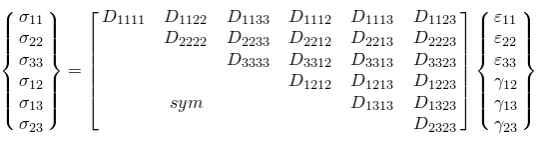 Abaqus's Constitutive relations
 SwiftComp's Constitutive relations
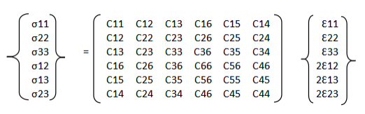 SwiftComp's output Constitutive relations converted into Abaqus's input Constitutive relations
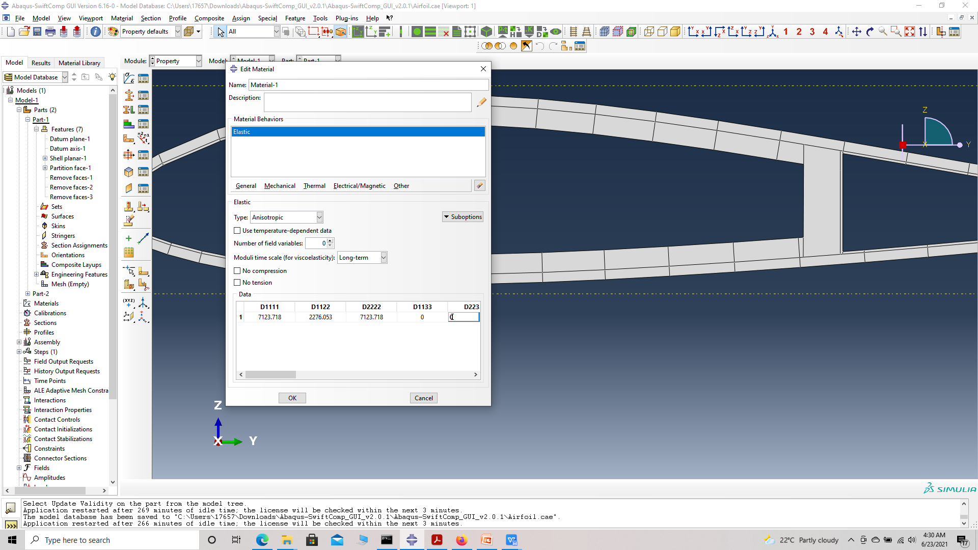 Importing Material properties
# Step 3.4. Now go to New Layups and add the material, section name, Layup and thickness to create the required layup. This is repeated five time since we have multiple layups. We will use plies of orientation 0,45 and -45 with a individual ply thickness of 0.1 mm for all laminates of the Airfoil. We will also have to portion the web as shown in part-1 model tree -> partition face->edit section sketch -> make appropriate changes -> Feature -> Regenerate.
Layup 1 – (0/45/-45/0)s
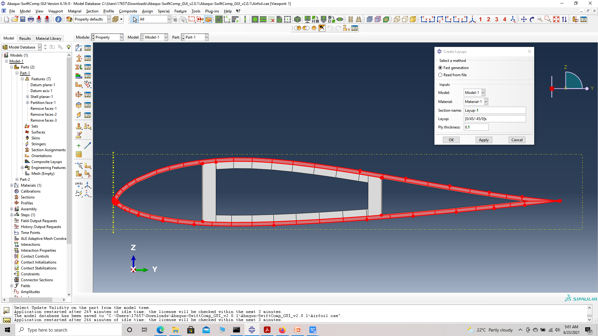 Layup-1
Layup 2 – (0)2
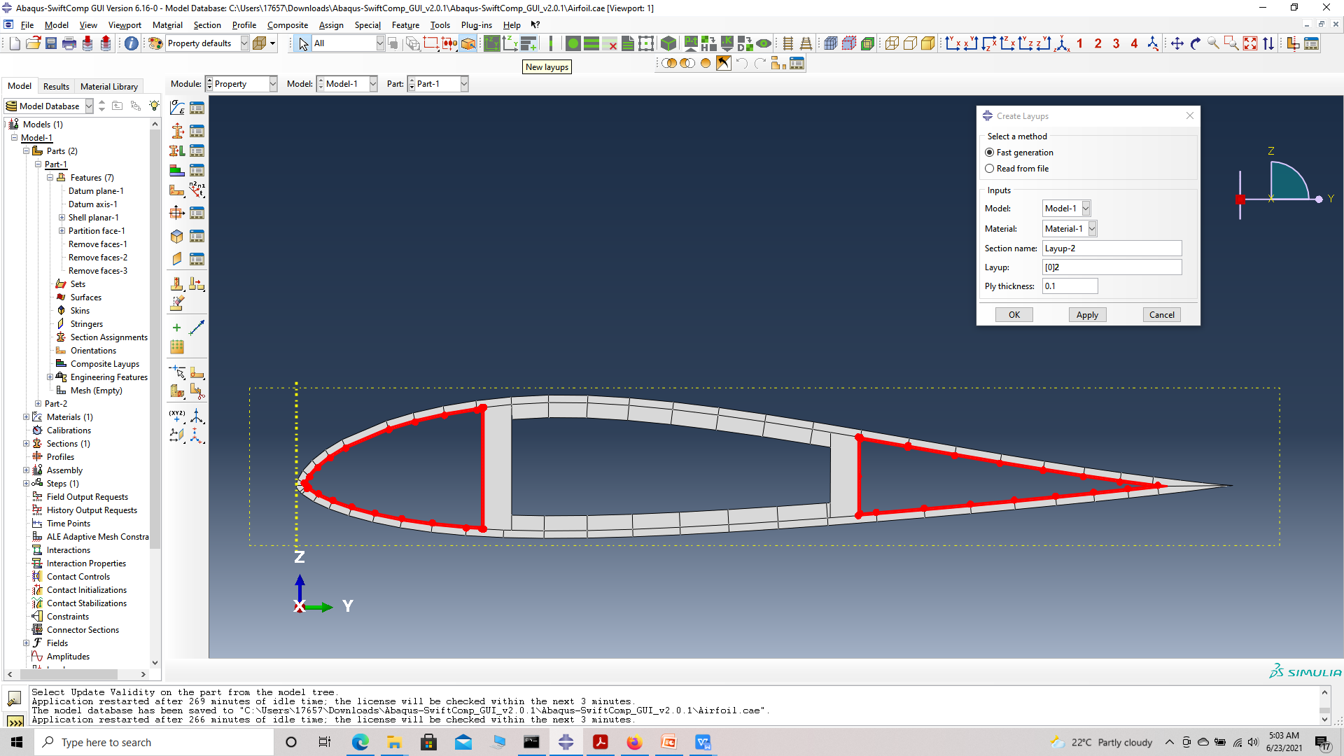 Layup-2
Layup 3 – (0/45/-45/0)2s
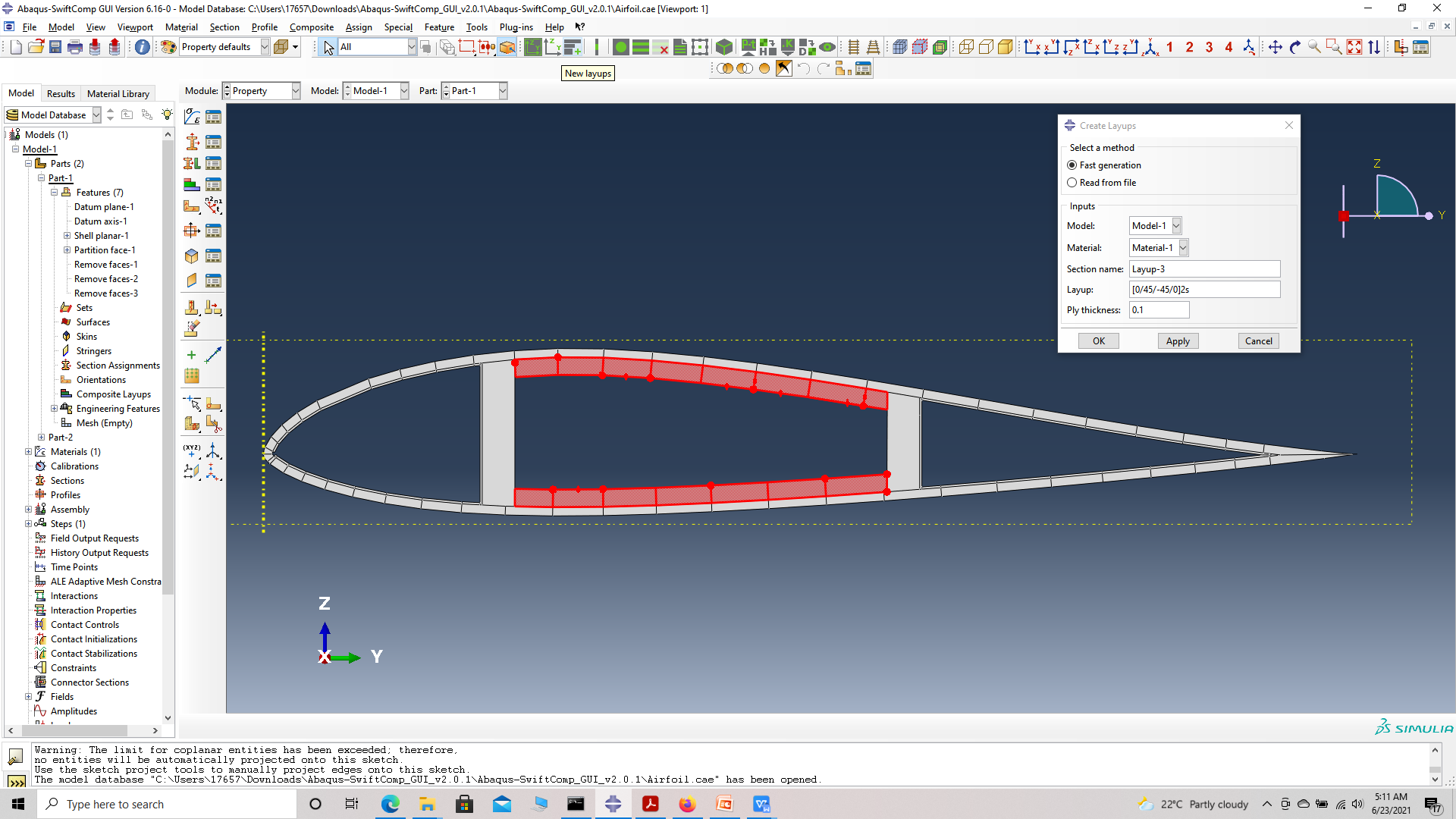 Layup-3
Partition part
 edit partition
 New partition
Layup 4 – (0/45/-45)2s
 Layup-4
Layup 5 – (0)6
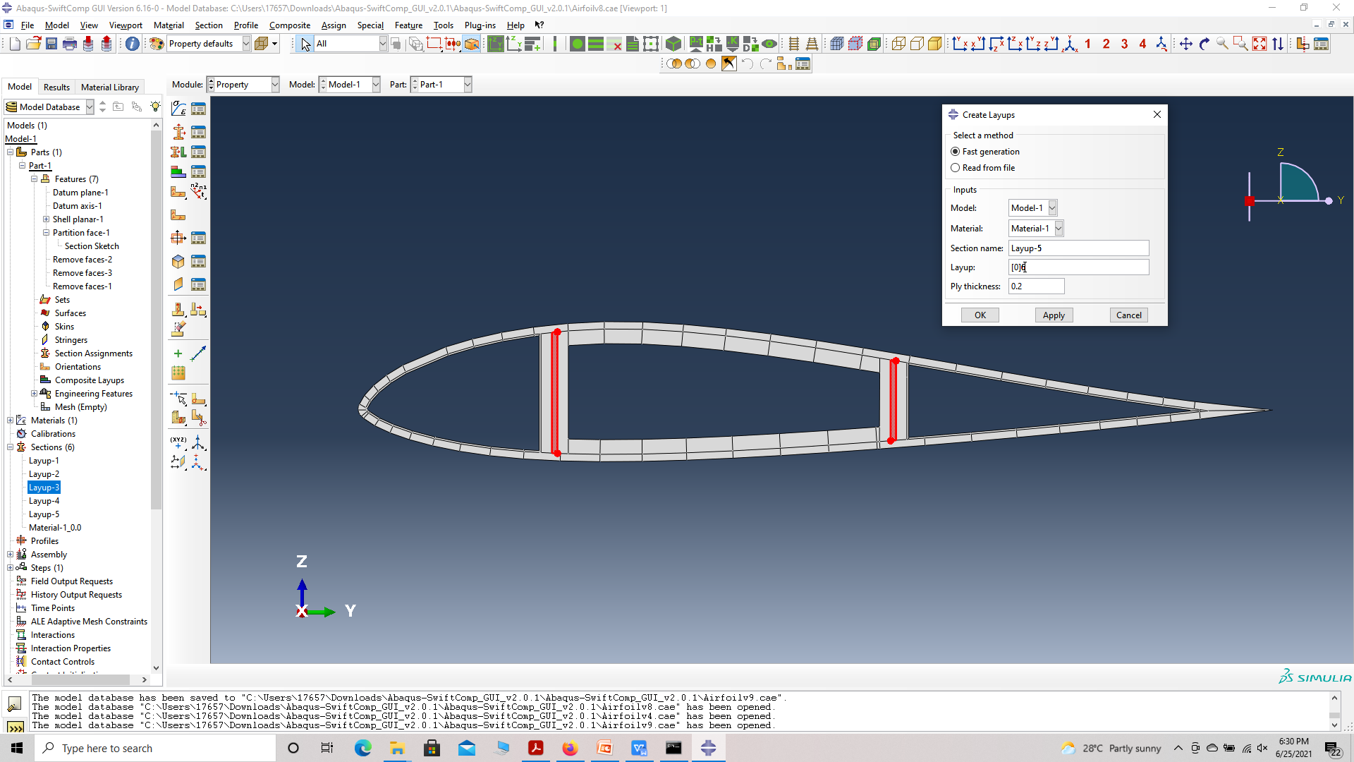 Layup-5
‘ # Step 3.5. To assign the layup, go to Create 2D SG: Assign Layups and the pick the baseline, the line opposite to the baseline and the area between the two picked line for the section as shown and then hit Ok. Do this for all sections. Since we have reduced the model, we will consider the outer lines as base lines
 Assign Layups
 Assign Layups
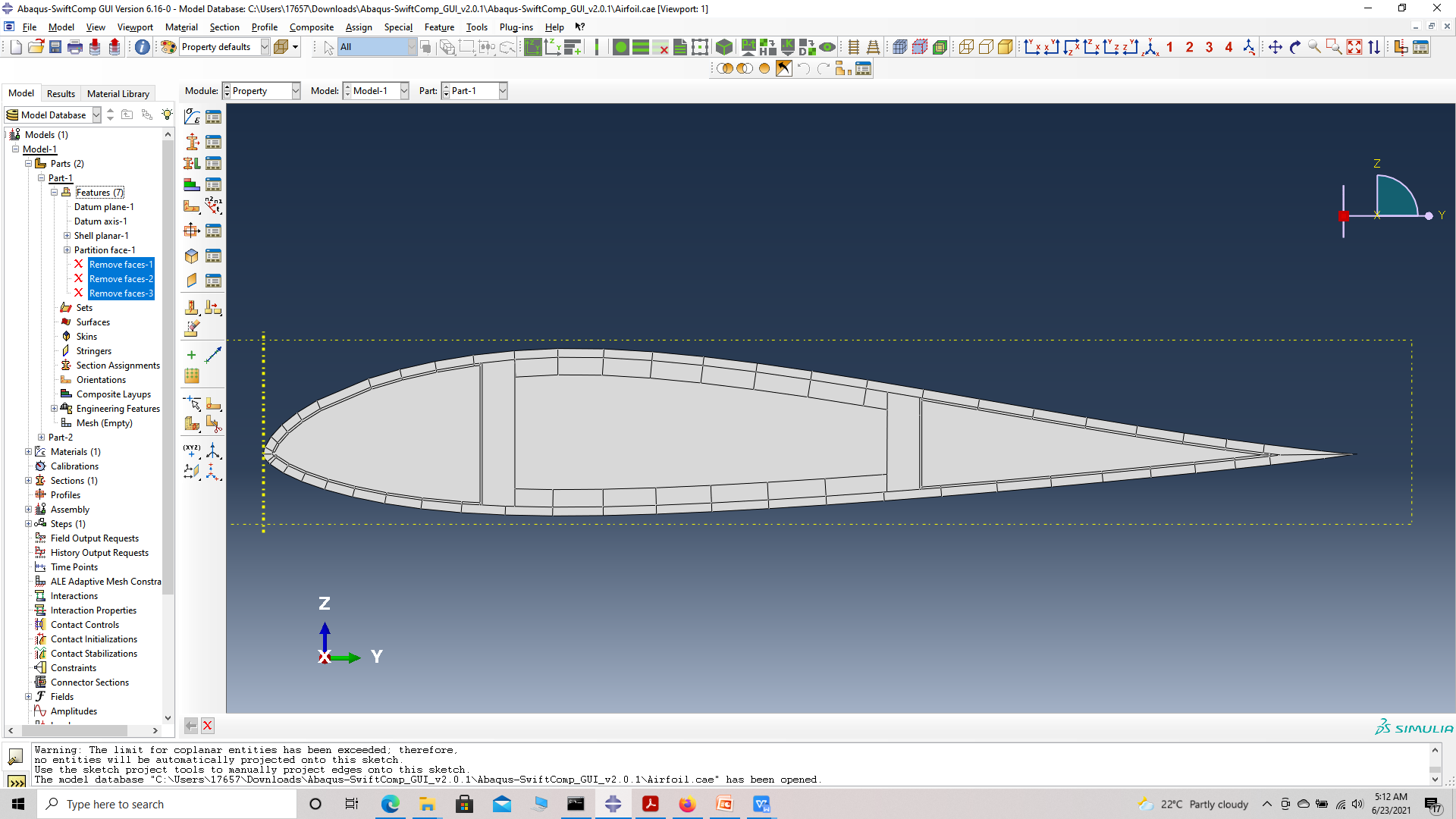
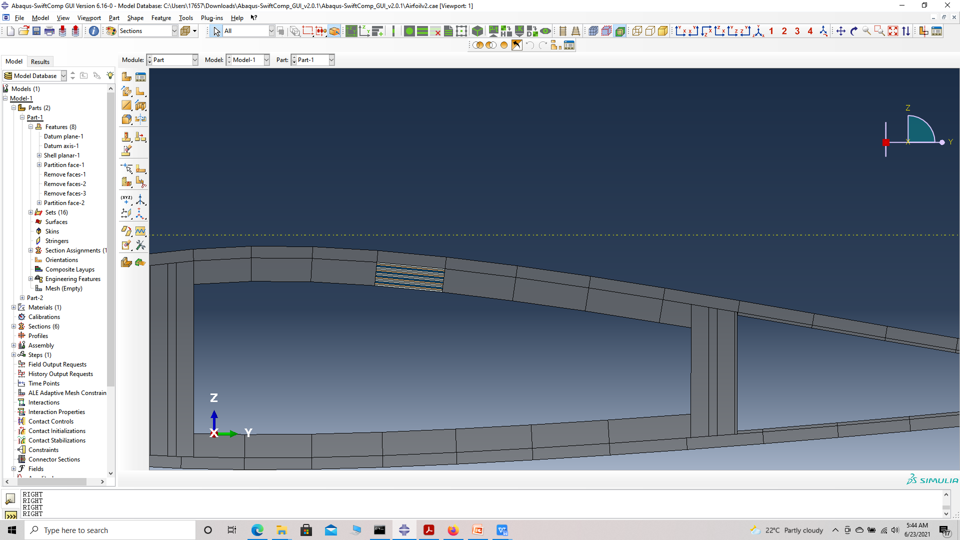
# Step 3.6. We can also partition the part and assign materials manually, which is another time consuming option. Since the add layup feature uses regenerate option each time a new layup is assigned, the limited computational resources of the free student edition of abaqus will direct this tutorial to use the manual partition method with half the plies, ie the ply thickness is increased to 0.2 mm. So the final part with the layups assigned will resemble the figure below.
 Assign Layups
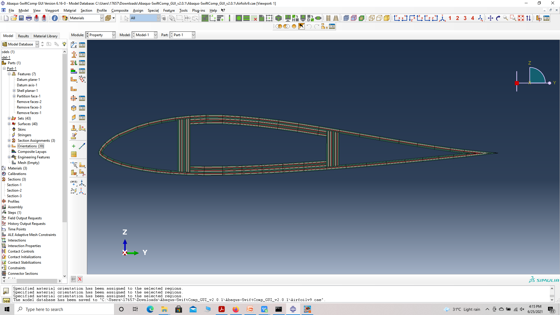
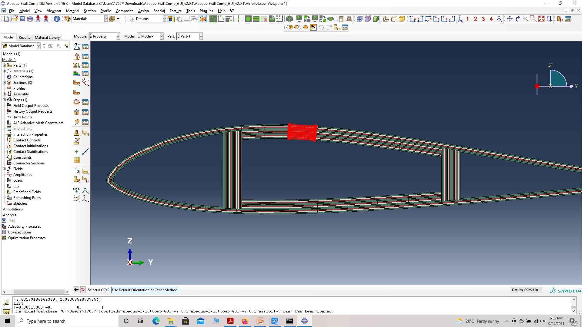
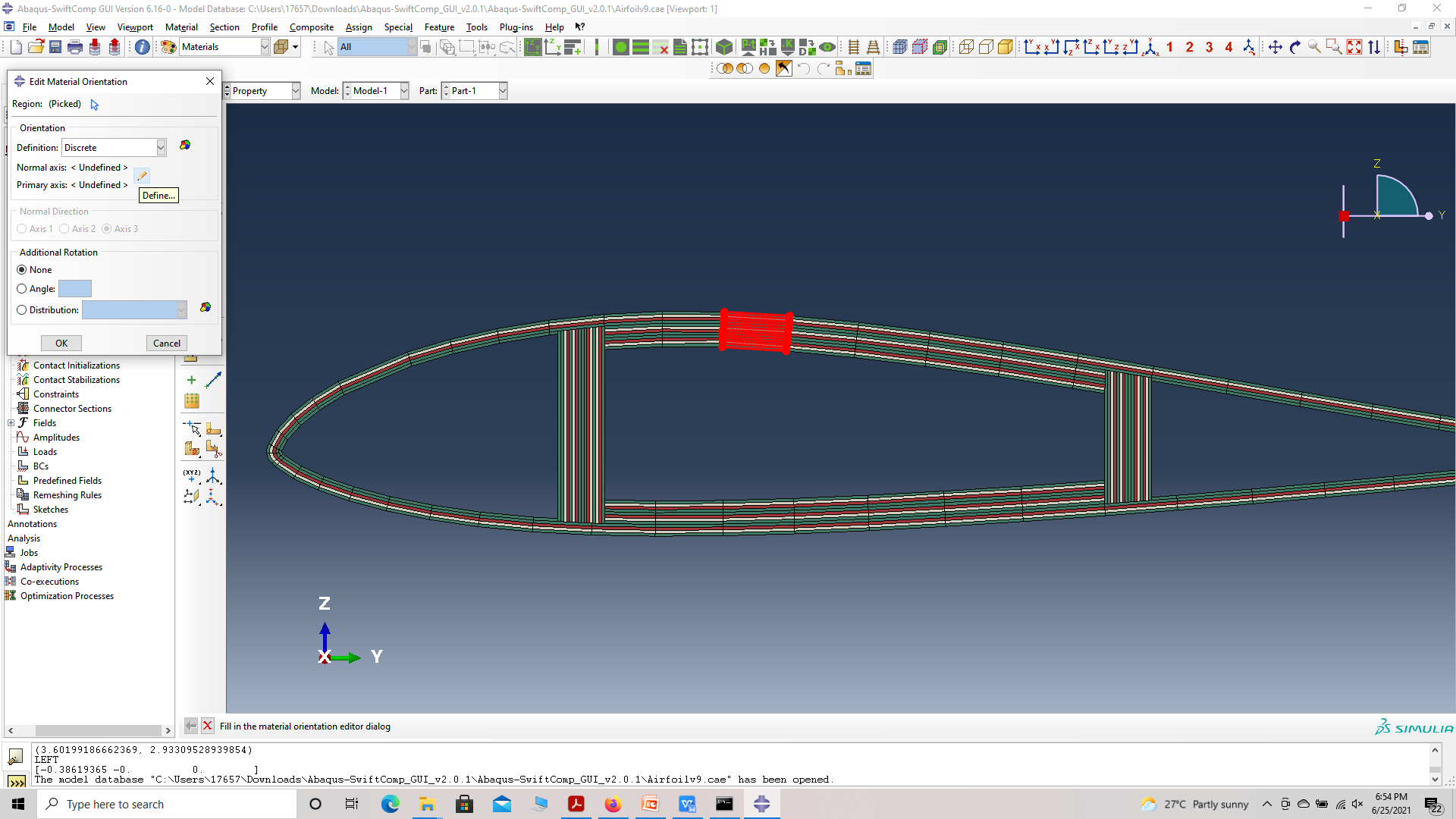
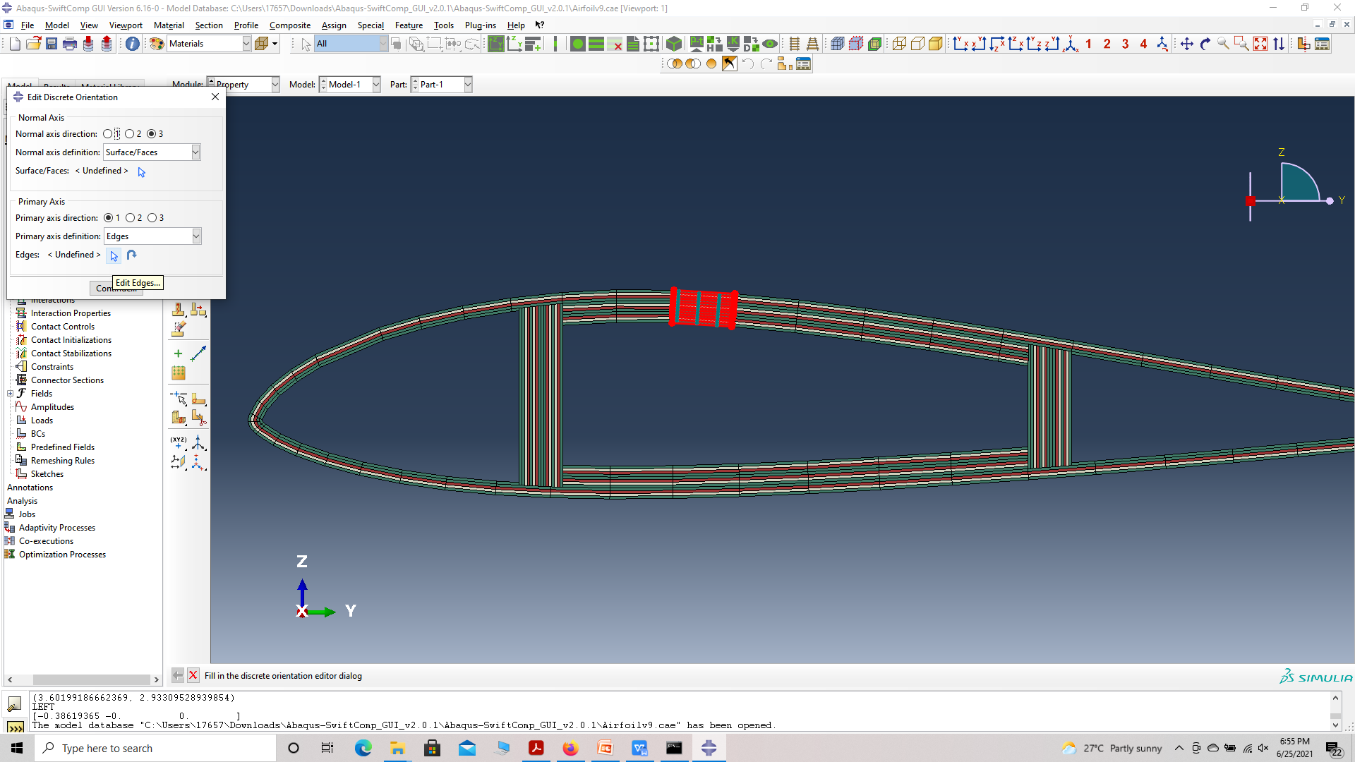
‘ # Step 3.7. Now we assign the material orientation for the part. Go to Assign material orientation -> select the sections of the part with the same orientation -> Done -> Select a CSYS (use default orientation or other method) -> Definition (Discrete) -> Define -> Primary axis orientation -> choose edge and flip direction if needed to make the axis point towards a clockwise direction -> Choose the surfaces for the normal axis definition -> Continue -> OK. Orientation Axis 1 represents the y2 axis of SwiftComp’s local orientation and orientation axis 2 represents y3 axis of SwiftComp’s local orientation.
 Assign material orientation
 Select a CSYS
 Define orientation
 edit edges
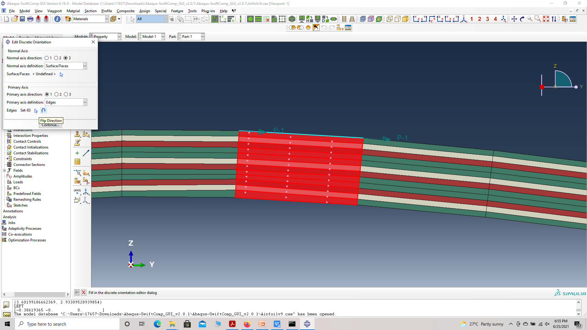 flip edges to clockwise orientation
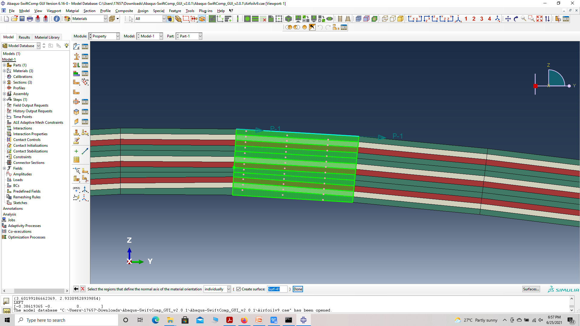 choose surfaces
 Orientation
 Part Orientation
‘ # Step 3.8. Now go to Assemble, create the part instance with dependent mesh.
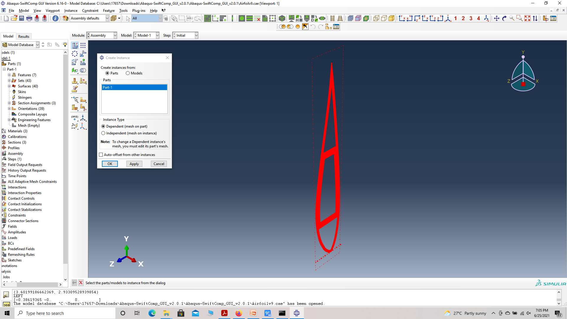 assembly
# Step 3.9.In the Mesh section, Seed the Part and set approximate global mesh size, then Click ‘Mesh Part’
 Mesh
Mesh
# Step 3.10.Create a job and write its input file.
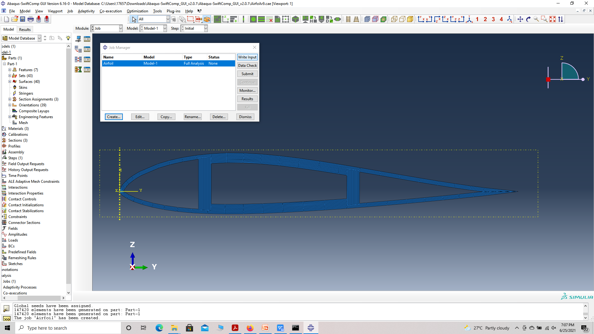 ip file
# Step 3.11.To the effective elastic properties. we click on Homogenization and select elastic in Analysis Type. Homogenize the part preferably as a beam using the Homogenization via input file option to get the final results.
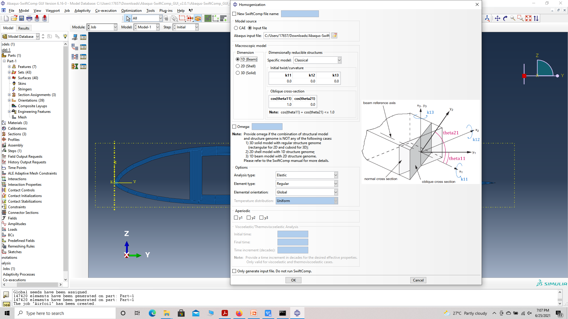 Homogenization
References
# Chen, H., Yu, W. & Capellaro, M. A critical assessment of computer tools for calculating composite wind turbine blade properties. Wind Energy, 13, 497-516, 2010.