Problem Description
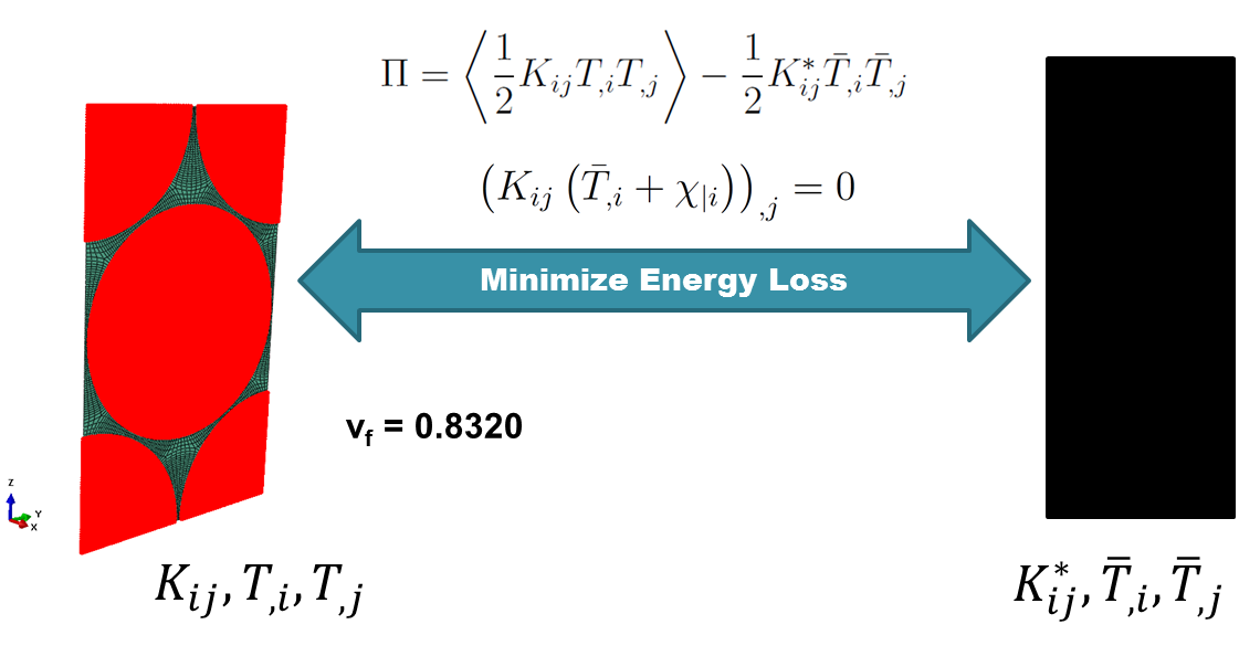
Homogenization Problem
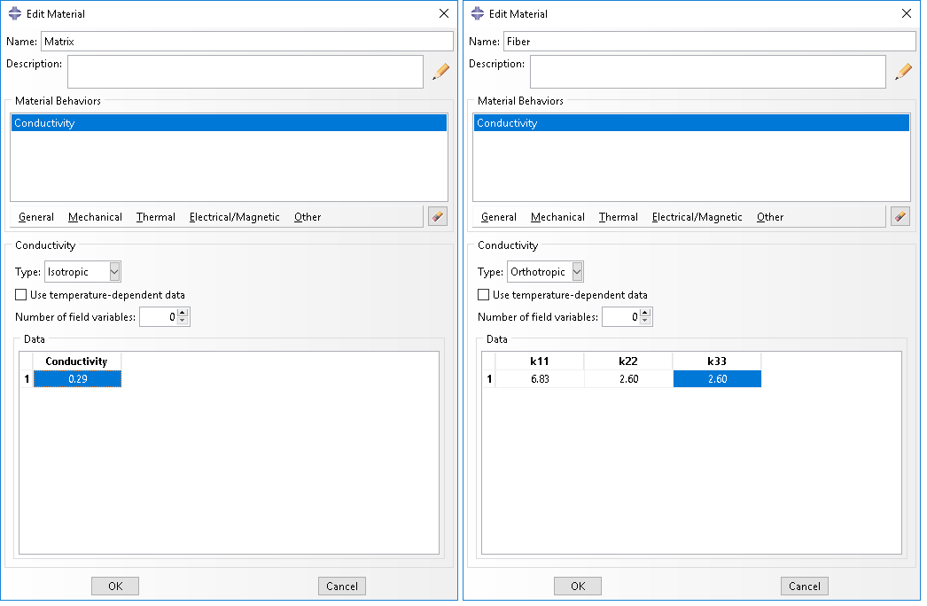
In this example, isotropic matrix and transversely isotropic fiber are considered as constituent materials and we want to compute the effective thermal conductivity of the composite material. The corresponding material properties that we will use are defined in the following table.
| Resin Conductivity, kr | 0.29 W/m/K |
| Fiber Conductivity in Fiber Direction, kf11 | 6.83 W/m/K |
| Fiber Conductivity in Transverse to the Fiber Direction, kf22 | 2.60 W/m/K |
We will use a hexagonal pack with fiber volume fraction equal to vf = 0.8320
 Homogenization process
Software Used
In his tutorial we will use Abaqus CAE with the Abaqus SwiftComp GUI plug-in. Abaqus CAE will be used to define the material properties and Abaqus SwiftComp GUI to define the different structure genomes (SGs). SwiftComp will run in the background.
Solution Procedure
The steps required to compute the effective thermal conductivity using Abaqus SwiftComp GUI are as follows.
# Step 1. We define the material properties in global coordinate system. In this case, we only need to define thermal conductivity properties in Abaqus CAE clicking on Thermal, Conductivity.
 Definition of thermal conductivity as constituent properties
# Step 2. From the default the Abaqus SwiftComp GUI SGs, we pick the 2D Structure Genome with Hexagonal pack.
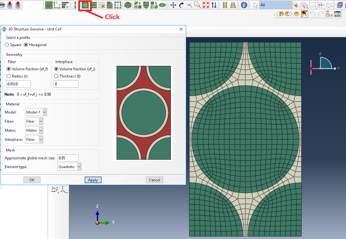 Definition of the 2D SG hexagonal pack microstructure
# Step 3. Now, in order to compute the homogenized thermal conductivity properties, we click on Homogenization and we select Conduction in Analysis Type.
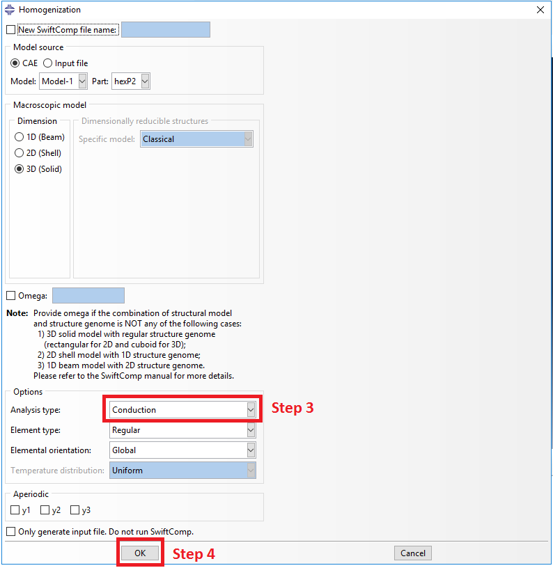 Definition of the homogenization step
# Step 4. We click on Ok to run the homogenization step. SwiftComp on the background will run the homogenization.
 SwiftComp running on the background
# Step 5.The results can be found in the .sc.k file as shown next. Note that the first matrix corresponds to the effective thermal conductivity matrix in the form of Kij*. The second matrix corresponds to the compliance matrix in the form of (Kij* )-1.
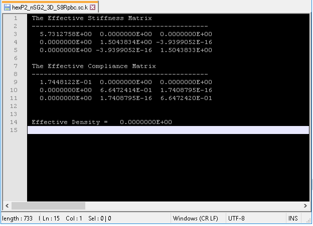 Results corresponding to the effective thermal conductivities
References
- Rique, O.; Barocio, E.; Yu, W.: “Experimental and Numerical Determination of the Thermal Conductivity Tensor for Composites Manufacturing Simulation,” ASC 32nd Technical Conference, October 2017, Purdue University.