Problem Description
Homogenization Problem
This tutorial shows how to calculate cross-sectional properties of the Lenticular boom with given dimensions and material properties using SwiftComp 1.3 and SwiftComp Abaqus GUI.
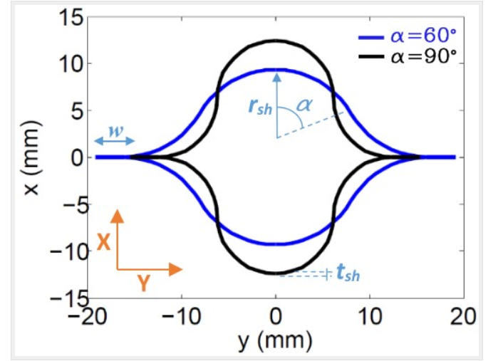 Flattened height: 45 mm, Web height(one side): 3 mm, Subtended angle: 90 degree, Ply thickness: 0.04 mm,
Radius of the flange (curved part): 6.21 mm,
Layup: (30)2 . The layup sequence is along with the direction pointing to the center of flange.
Flattened height: 45 mm, Web height(one side): 3 mm, Subtended angle: 90 degree, Ply thickness: 0.04 mm,
Radius of the flange (curved part): 6.21 mm,
Layup: (30)2 . The layup sequence is along with the direction pointing to the center of flange.
In this example, isotropic matrix and transversely isotropic fiber are considered as constituent materials and we want to compute the effective thermal conductivity of the composite material. The corresponding material properties that we will use are defined in the following table.
| Resin Conductivity, kr | 0.29 W/m/K |
| Fiber Conductivity in Fiber Direction, kf11 | 6.83 W/m/K |
| Fiber Conductivity in Transverse to the Fiber Direction, kf22 | 2.60 W/m/K |
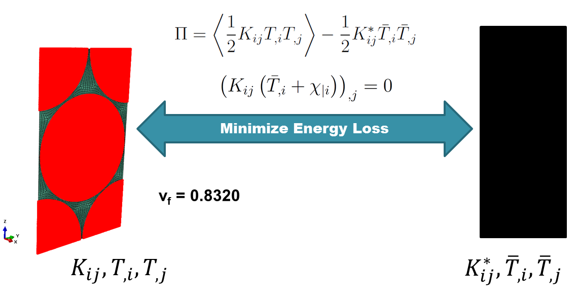
We will use a hexagonal pack with fiber volume fraction equal to vf = 0.8320
 Homogenization process
Software Used
In his tutorial we will use Abaqus CAE with the Abaqus SwiftComp GUI plug-in. Abaqus CAE will be used to define the material properties and Abaqus SwiftComp GUI to define the different structure genomes (SGs). SwiftComp will run in the background.
Solution Procedure
The steps required to compute the effective thermal conductivity using Abaqus SwiftComp GUI are as follows.
# Step 1. We define the material properties in global coordinate system. In this case, we only need to define thermal conductivity properties in Abaqus CAE clicking on Thermal, Conductivity.
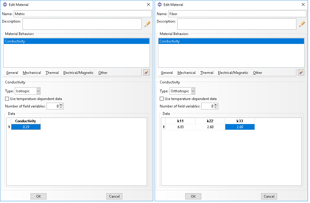 Definition of thermal conductivity as constituent properties
# Step 2. From the default the Abaqus SwiftComp GUI SGs, we pick the 2D Structure Genome with Hexagonal pack.
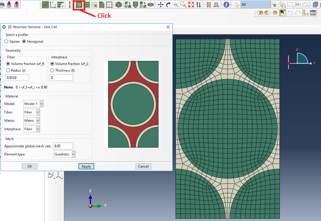 Definition of the 2D SG hexagonal pack microstructure
# Step 3. Now, in order to compute the homogenized thermal conductivity properties, we click on Homogenization and we select Conduction in Analysis Type.
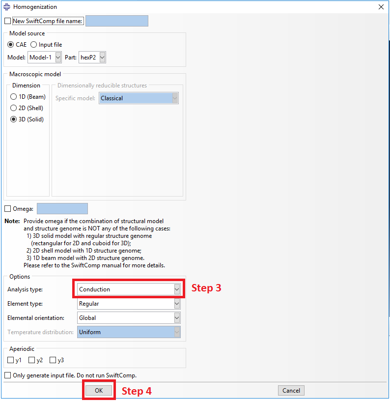 Definition of the homogenization step
# Step 4. We click on Ok to run the homogenization step. SwiftComp on the background will run the homogenization.
 SwiftComp running on the background
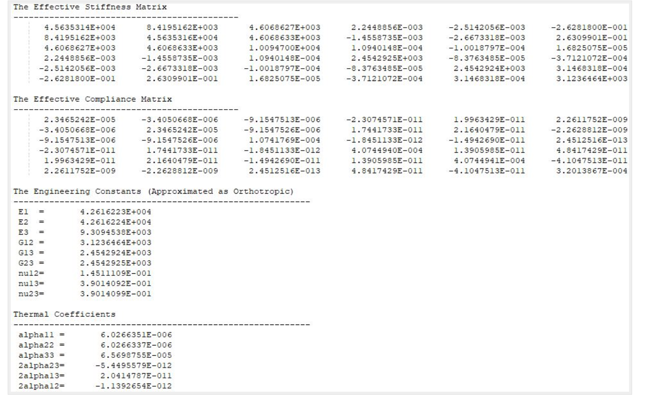
# Step 5.The results can be found in the .sc.k file as shown next. Note that the first matrix corresponds to the effective thermal conductivity matrix in the form of Kij*. The second matrix corresponds to the compliance matrix in the form of (Kij* )-1.
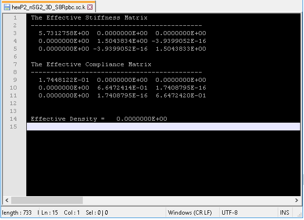 Results corresponding to the effective thermal conductivities
The MSG solid model is used to predict the effective thermoelastic properties of a plain weave composite by taking the effective yarn properties and matrix properties to predict the effective properties of weave composites. Software Used
The example will be solved using the TexGen4SC 2.0. Solution Procedure
Below describe the detailed step by step procedure you followed to solve the problem.
# Step 6 Create mesoscale plain weave SG with the yarn geometries given as
# Step 7 Create plain weave pattern as
# Step 8 Go to Homogenization->Microscale and select thermoelastic analysis. Keep the default material properties. The fiber volume fraction 0.64 as
 Click finish and the microscale homogenization will be performed and the results will be automatically pop up. Note
# Step 9 The effective yarn properties will be automatically assigned to the mesoscale model. However, users need to define the matrix properties for the mesoscale model. Usually, the matrix at the mesoscale is the same as the one at microscale as shown
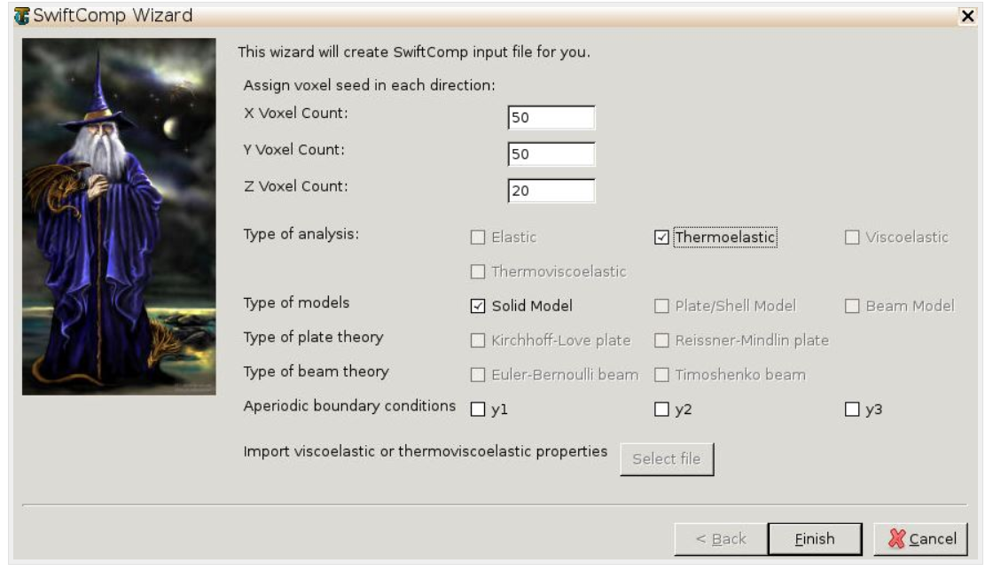
# Step 10 Go to File->Export->SwiftComp File, define the voxel mesh and run elastic analysis using the MSG solid model
 Save the sc file and click to the Homogenization->Mesoscale. The effective properties of the plain weave composite will be automatically pop up
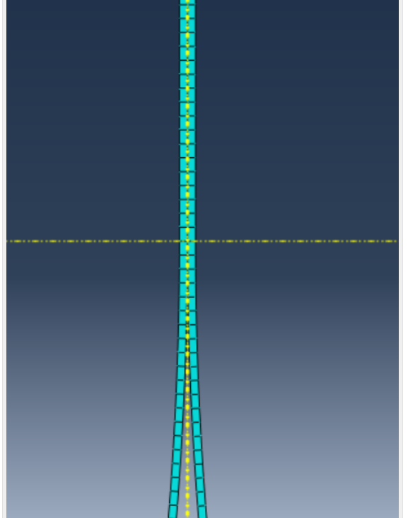
- Step 11 .We move on to macroscopic homogenization of the Lenticular boom.
(Image(l188.PNG) failed - File not found)
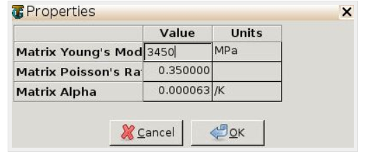
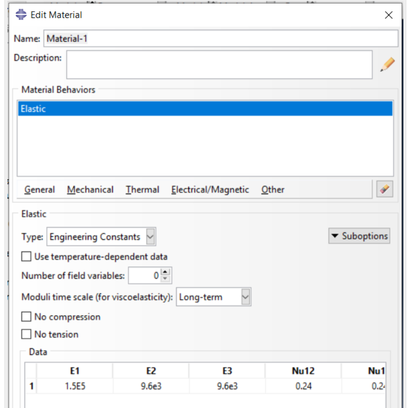
# Step 12.Go to Module > Property > Create Material and create a material with the properties obtained in the previous step.
# Step 13.’We move on geometry and create the cross section from Module > Property > Create Section . Create a section, Layup-1, shown as below with Solid-Composite. Note here that the thickness of each layer should be actual thickness instead of relative thickness.
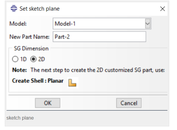
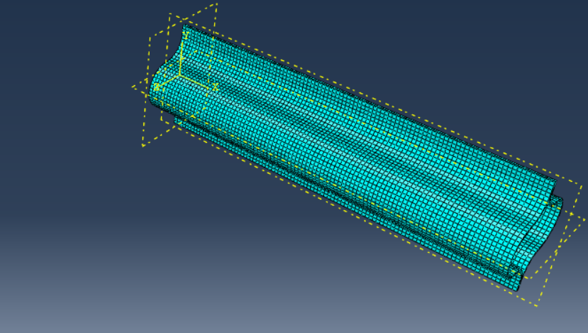
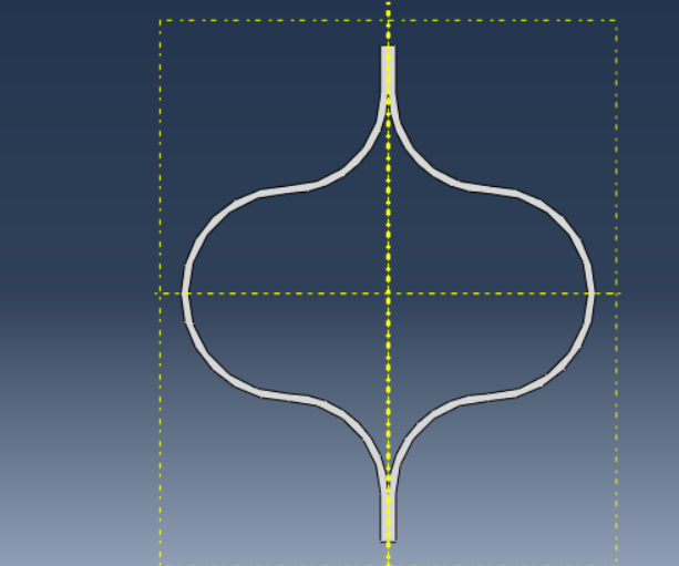
# Step 14.To create the geometry, in the SwiftComp Toolset, click the “Set sketch plane for 1D/2D customised SG” and secelt the 2D option. In the toolbox of the Part module, click ‘Create Shell: Planar’ , following the prompt, select the datum plane and the datum axis. Sketch the shape shown below. Click ‘Done’, then the part will be generated sketch planesketch plane
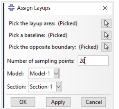
# Step 15.First we will assign the layup for the segment on the right. Make the two partition as shown and Click ‘Assign Layups’ in the SwiftComp toolset. Pick the area in the right, pick the appropriate baseline and select section ‘Layup-1’. Click ‘OK’. Repeat the step for all segments.
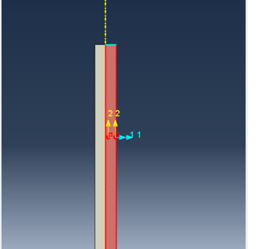
# Step 16.To assign local coordinates, go to Module > Property > Assign Material Orientation Following the prompt, we first select the top segement to be assigned a local material orientation, and click ‘Done’. Then in the prompt area, click ‘Use Default Orientation or Other Method’ button. In the ‘Edit Material Orientation’ dialog box, select ‘Discrete’ as the Orientation Definition. Then click , open the ‘Edit Discrete Orientation’ dialog box. In the Normal axis definition choose Vector (i,j,k), and set the vector (1.0, 0.0, 0.0). For Primary Axis, choose 1 as the Primary axis direction and Edges as the Primary axis definition. Click to select the light blue edge shown in the figure below, then click ‘Done’. Use Flip Direction to make the axis pointing to the right if necessary. Click ‘Continue…’ then ‘OK’ to finish this assignment. Same procedure for the rest three segments. Some steps may not be exactly the same. The only requirement is to make sure that the asix 2 pointing outwards.
material orientation
 # Step 17. Module > Mesh > Seed Part and choose mesh size, then Click ‘Mesh Part’
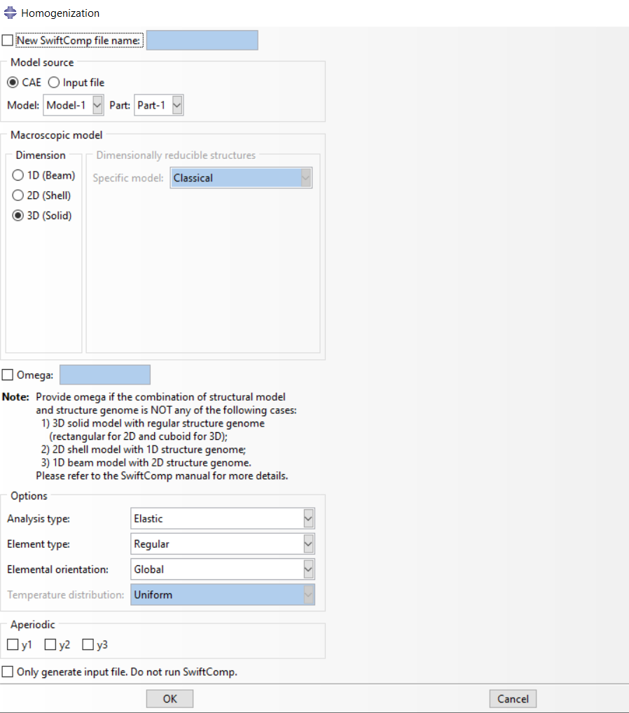
 # Step 18. Homogenize the part to get the final results.