Prof. Yu's Research Group in the Cloud

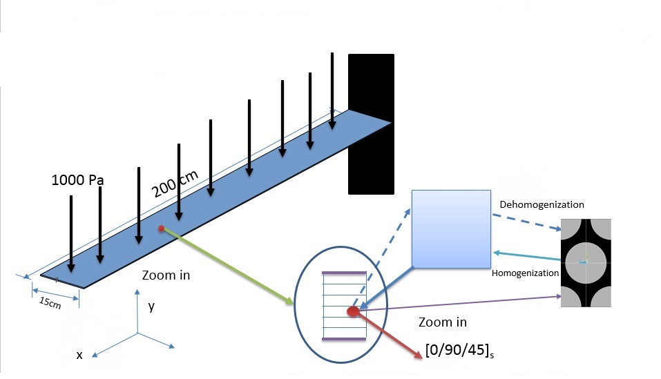
In this problem, we will try to show how to analyze the local-global fields in composite structures using SwiftComp-Abaqus-GUI.
The figure below can summarize how to do the local global analysis.

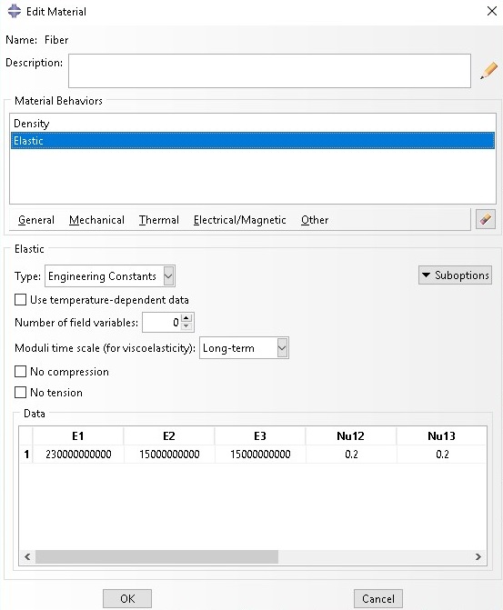
Let the material properties a fiber (T300) property be: : E₁₁=230 GPA, E₂₂=15 GPA, v₁₂=0.20, v23=_0.0714, G₁₂=15GPa, G₇=3.928GPa.
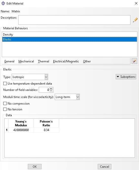
and matrix (3501-6 epoxy) be: E =4.2GP, ν=0.34
The composite lay-up:

[0/90/45],,s,,

Thickness of each ply=0.00025m

“Soden, P. D., Hinton M. J. and Kaddour, A. S., Lamina properties, lay-up configurations and loading conditions for a range of fibre reinforced composite laminates. Compos. Sci. Technol., 1998, 58(7), 1011”

Major steps to perform local-global analysis

Step 1: Input material properties

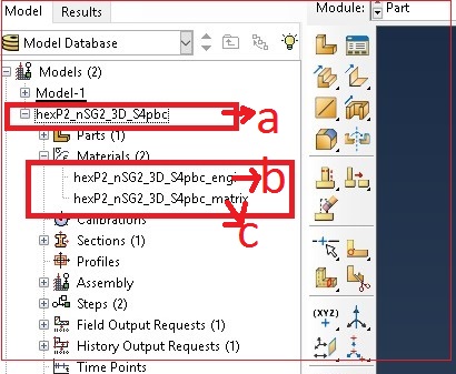
There are two materials namely fiber and matrix
a. Fiber properties
b. Matrix properties

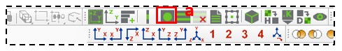
Step 2: Select appropriate SG

a. Select 3D SG that represent the current example

b. 3D SG wizard shows up
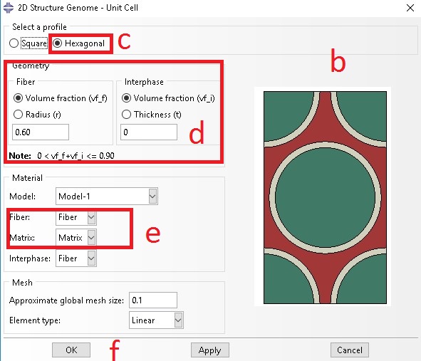
c. Select spherical inclusion as microstructure
d. Add inclusion volume fraction
e. Select material properties for inclusion and matrix
f. Click on OK to generate the SG
g. See generated 2D SG
(Image(Problem-4bb.JPG) failed - File not found)
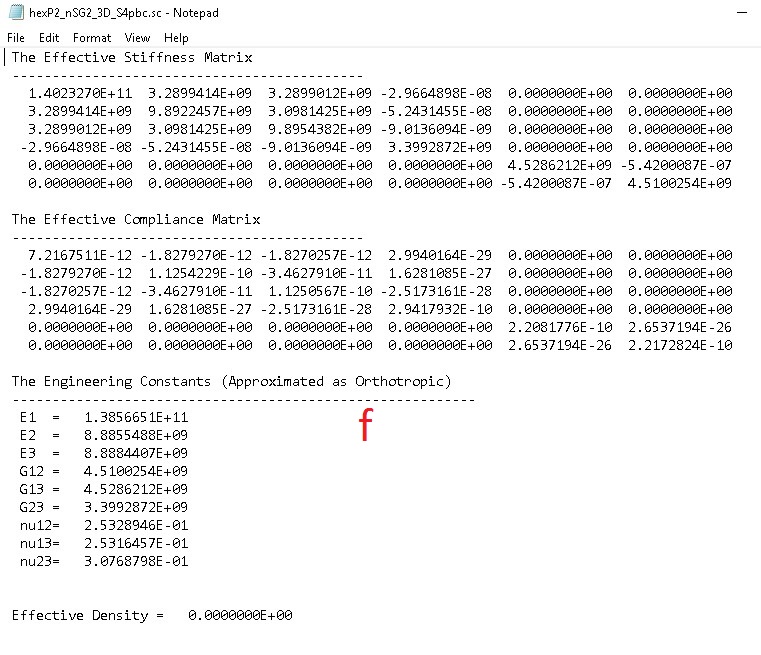
Step 3- Homogenization- 3D effective properties
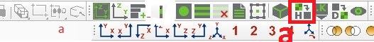
a. Click on Homogenization

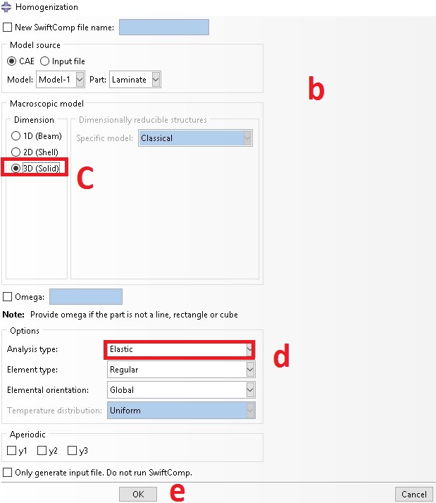
b. Homogenization wizard shows up ( see below)
c. Select 3D (solid) Model
d. Select analysis type, elastic
e. Click on OK to start homogenization
f. See the predicted 3D effective properties

Step 4: Export predicted effective properties to create a new model
a. Export the predicted effective properties

b. A new model is automatically generated, this is to be used for generating a global model
c. Predicted effective properties exported as engineering constants
d. Predicted effective properties exported as stiffness matrix, D,

Step 5: Generate the global model
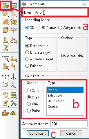
a. Click on Part and name as Part-1
b. Select ‘Shell’ from from Shape and ‘Planer’ from type
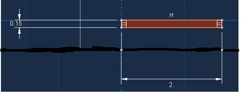
c. A new model is generated as shown ( 0.2m and thickness=0.15m)


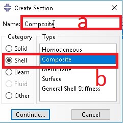
Step 6: Create and Assign Section’
a. Click on Section and name as ‘Composite’
b. Select ‘Shell’ from from Category and ‘Composite’ from type
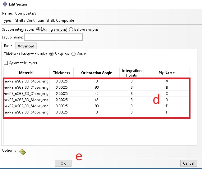
c. Edit section wizard shows up
d. Add section properties as shown and click OK


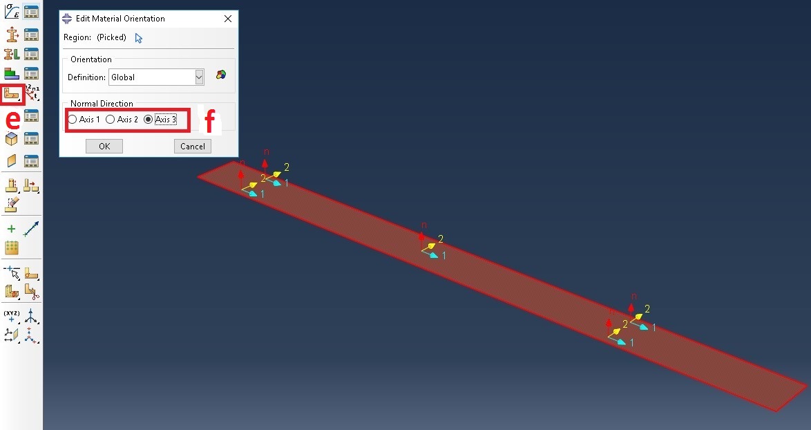
e. Assign material orientation
f. Click on Axis 3

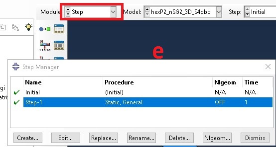
Step 7: Create Assembly and Steps ‘
a. Select Assembly
b. Select ‘Part-1’ from Create Instance
c. Click OK
(Image(Problem-4M7.jpg) failed - File not found)
e. Create steps, accept the default setting

Step 8: Create load and boundary conditions ‘
a. Select load from Module
b. Select load
c. Name the load as ‘Load-1’
d. Select step 1
e. Select pressure


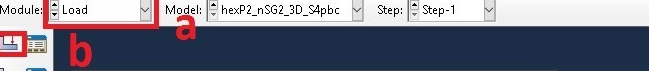
f. Select the area to be loaded
g. Add the load
youtube link:
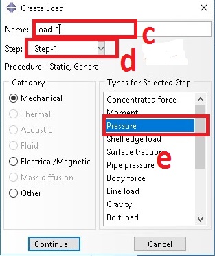
Step 9: Create boundary conditions ‘
a. Select load from Module
b. Boundary Conditions (BC)
c. Name the BC as ‘BC-1’ and Select ‘Step-1’
d. Select ‘Mechanical’ from Category and Symmetry type BC
e. Click on OK

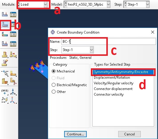
f. Select the edge for BC
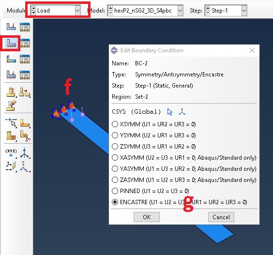
g. Select ENCASTER

Step 10: Create Mesh ‘

Step 11: Run the analysis ‘

Step 11: Results of the analysis ‘

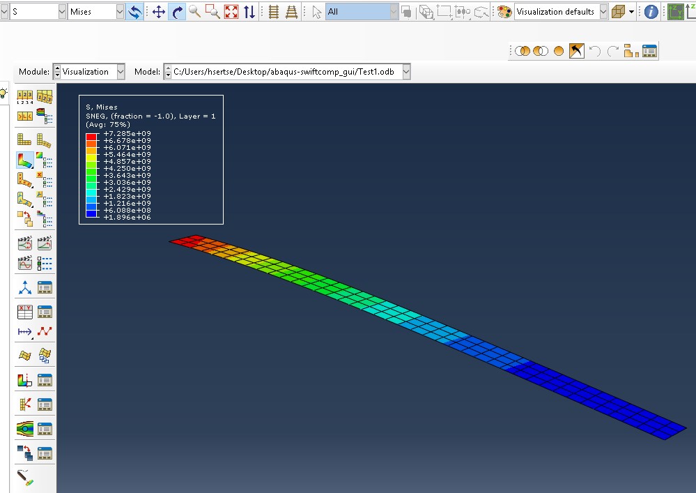
Step 12: Obtain global strains ‘
a. Click on probe values to obtain global strain
b. Click on a point on global structure
c. Select nodes and all direct from probe values wizard
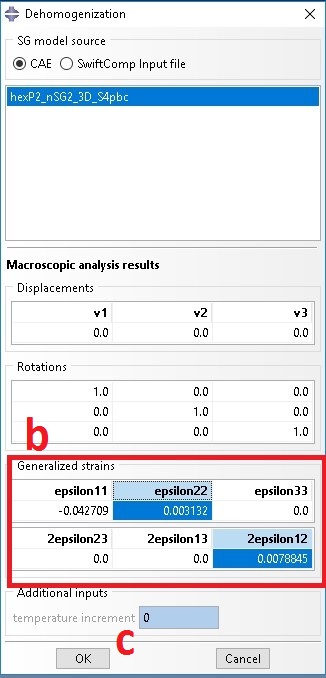
d. The following strain values can be obtained, strain e₁₁=-0.042709, e₂₂=0.00212116, 2e₁₂=0.00788458, and all others are zero
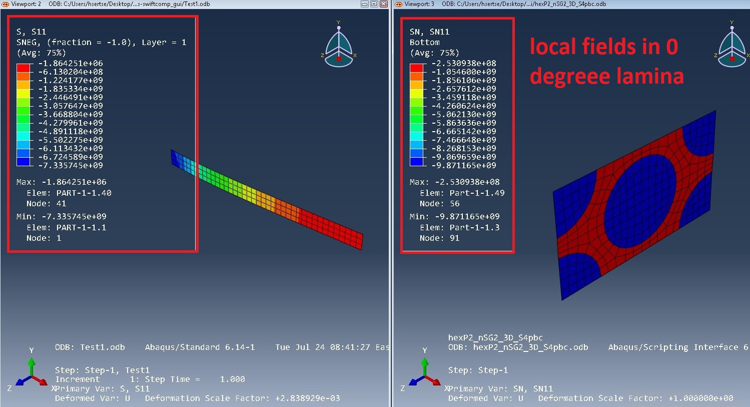
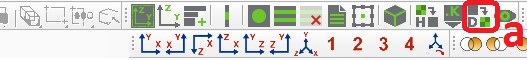
Step 13: Run dehomogenization ‘
a. Go back to micromechanical analysis with hexagonal SG and click on dehomogenization

b. Add global strain obtain in step 12 to obtain local field in 0 degree lamina
C. Click on OK

Step 14: Create view port and show both global and micromechanical local field analysis ‘

Created on 25 Jul 2018, Last modified on 27 Jul 2018