Problem Description
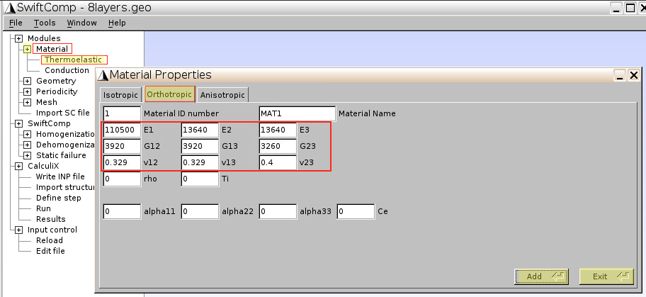
A simple composite laminated beam as shown in Fig.1 is clamped at x=0, and subjected to a 10 kN point force in x-direction and a 10 kN∙mm moment in y-direction at x=1m. Dimensions of the beam and layup of the laminate are given in Fig.1. The laminate is made of 8 layers, each of a continuous fiber reinforced composite. The lamina constants are $$E_1 = 110.5 \text{GPa}, E_2 = E_3 = 13.64 \text{GPa}, G_{12} = G_{13} = 3.92 \text{GPa}, G_{23} = 3.26 \text{GPa}, \nu_{12} = \nu_{13} = 0.329, \nu_{23} = 0.400. $$

Software Used
This wiki page is based on Gmsh4SC version 2.0.
A previous resource (Gmsh4SC Tutorial #1) including documents and Gmsh files, and the video are based on Gmsh4SC version 1.3.
Updates in tutorial for Gmsh4SC ver. 2.0:
• Draw point and line elements using commands
• CalculiX boundary conditions
Companion Video
Please refer to the YouTube video by Xin Liu showing the solution procedure using Gmsh4SC version 1.3.
Solution Procedure
Below describes the step-by-step procedure you followed to solve the problem. It is better to accompany this document with the companion youtube video.
1. Input Laminate Geometry and Lamina Material Properties
The structure genome (SG) for this laminated beam is the cross section of the laminate beam, because there is no heterogeneity along beam reference line. Here we input material properties of each layer using orthotropic model, and geometry information directly generated by laminate layup code.
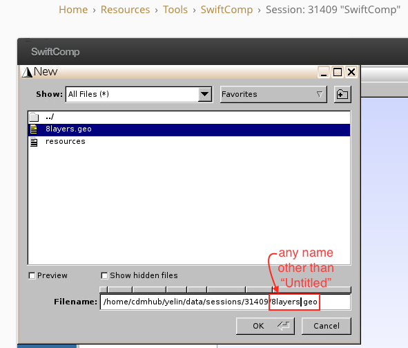
1.1 Create a new .geo file
- Click
File–New - Change the filename in
/path/to/current/session/Filename.geo(give a name other than Untitled)
1.2 Input lamina properties
- Click
Material–Thermoelastic–Orthotropic - Input the 9 lamina constants
- Click
Add–Close–Exit
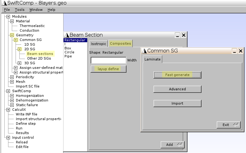
1.3 Input laminate geometry by composite layup
- Click
Geometry–Common SG–2D SG–Beam sections - Click
Composites–layup define–Fast generate
- Material:
1 -- MAT1(for lamina) - Layup:
[0/90/0/90]s(as shown in Fig.1) - ply thickness:
5(unit: mm, as total thickness for 8 layers is 0.04m)
 Fig5_GenLaminate_cont.gif
- Click
Add–Close, and get back to the previous window showing Beam Section – Composites - Width:
180(unit: mm, as shown in Fig.1), and clickAdd
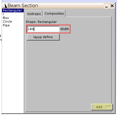
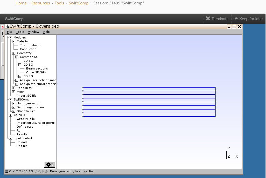
The geometry of the 8-layer laminate is generated.
2. Homogenization: Effective SG Properties Calculation
Now consider the 8 layers as a homogeneous material, we calculate the effective stiffness matrix of the SG by Homogenization command.
2.1 Mesh
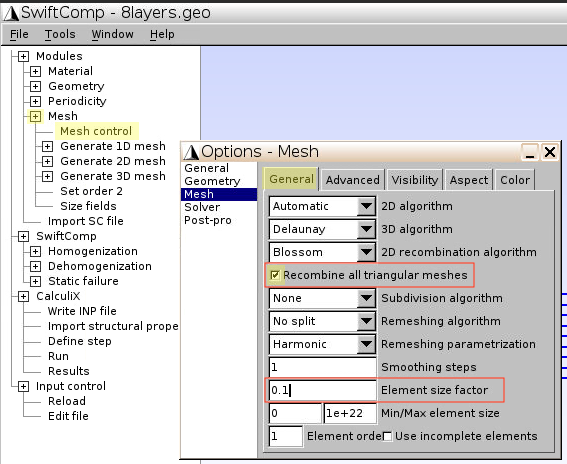
- Click
Mesh–Mesh control - In the
Generaltab, tickRecombine all triangular meshes, input Element size factor:0.1, then close this window
- Click
Generate 2D mesh–Generate, and you’ll see the mesh generated for 8 layers - Click
Set order 2
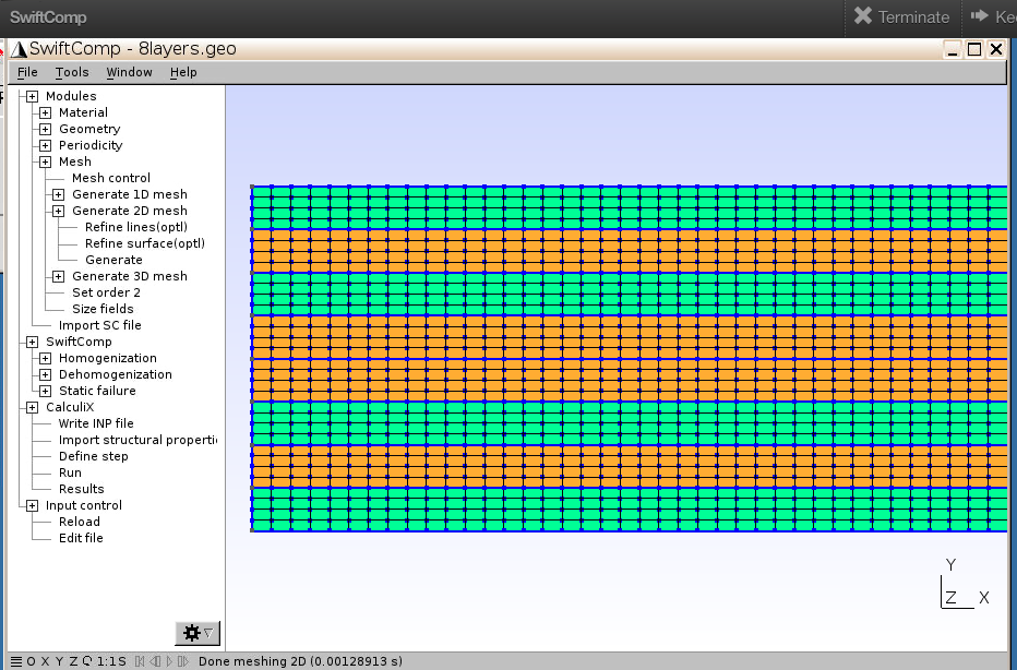
If you want to change mesh properties, e.g., change element size factor, you may reopen Mesh control, input the new number, and then click Generate again to get the new mesh.
2.2 Homogenization
- Click
SwiftComp–Homogenization–Beam Model - No need to change or input anything in this case
- Click
Save, wait for ~10 seconds, clickRun

2.3 Check results and save files
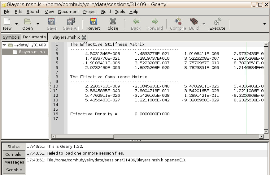
- Once the homogenization finishes, a plain text file
Filename.msh.kcontaining effective stiffness and compliance matrices of the laminate will pop up.
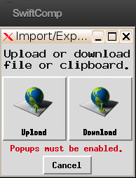
- You may download the files for your own record by the following methods.
- Use Import/Export tool on cdmhub. The tool is launched by default for every SwiftComp session.
- Use any FTP tool
- host:
cdmhub.org - username: if you forgot your username, it can be found in many ways. For example, if you’re logged on cdmhub webpage, on the upper right corner says “Logged in (
your_Username)”. Or, in any launched swiftcomp session, click the bottom grey bar or clickTools–Message Console, to show message console. On the 9th line it says “Info: Home directory: /home/cdmhub/your_Username/”. - password: same as your log in password to cdmhub webpage.
- remote site address:
/home/cdmhub/your_Username/data/sessions/5-digit_current_session_number - current session number can be found above the SwiftComp window, or in the title of the webpage, or in Dashboard – Activity.
- host:
- Use
sftpcommand line (the following commands work for Mac – Terminal)-
sftp your_Username@cdmhub.org -
get /home/cdmhub/your_Username/data/sessions/5-digit_current_session_number/Filename.msh.k local_folder_path - feel free to use
helpor?to check all available commands
-
- I usually download these files after homogenization:
- `Filename.geo`: geometry without mesh
- `Filename.msh`: geometry and mesh informations
- `Filename.msh.k`: results after homogenization
3. Macroscopic Analysis for the Beam
3.1 Create beam geometry
- Click
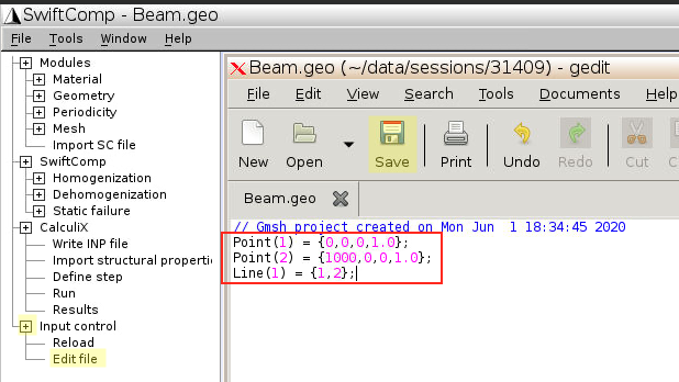
File–New, and input a different filename, e.g.,/home/.../Beam.geo, same as in Fig.2 - For Gmsh4SC version 2.0, you need to input the beam geometry by commands
- Click
Input control–Edit file - Manually add the following three lines:
Point(1) = {0,0,0,1.0}: create a point of position {x,y,z} = {0,0,0}, mesh size = 1.0
Point(2) = {1000,0,0,1.0}: create a point at x=1000 (unit: mm)
Line(1) = {1,2}: create a line connecting the two points.
- Click
Save, then close text editor
- Click
Reload, and you will see the beam geometry on the screen.

3.2 Input effective SG properties for the beam
- Click
Geometry–Assign structural properties–Beam, ClickClose
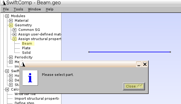
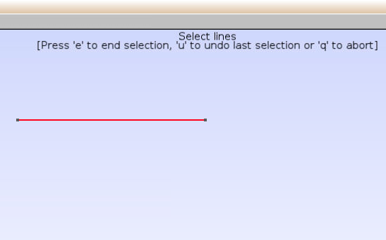
- Click on the red line, Press
eandq
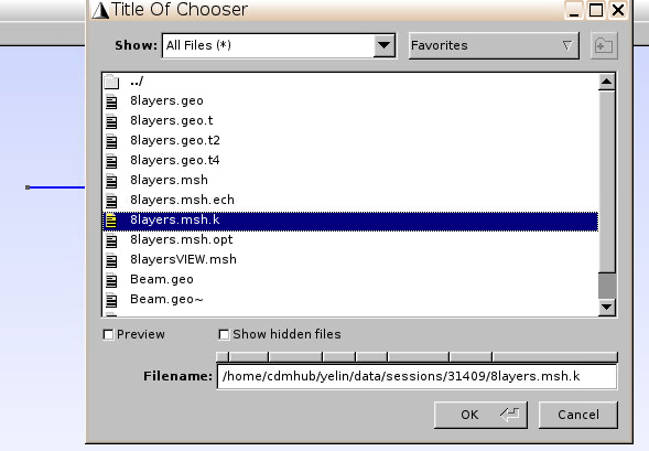
- In the pop-up browser window, choose
Filename.msh.k(the results file in Fig.11 after Homogenization step)
Now the beam is considered as a homogeneous material with effective material properties given in Fig.11.
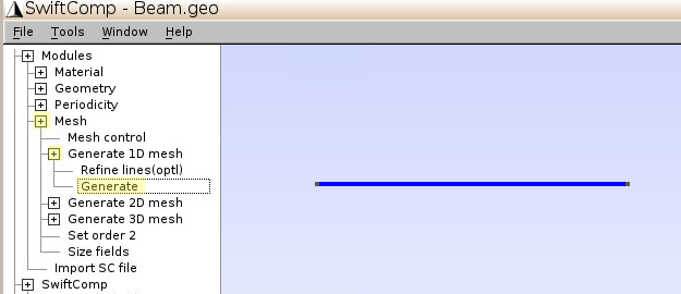
3.3 Generate mesh for the beam
- Change the elementary mesh size back to 1.0: Click
Mesh–Mesh control, input Element size factor:1.0 - Click
Mesh–Generate 1D mesh–Generate
3.4 Input file for CalculiX
- Click
CalculiX–Write INP file, to create the input file (Filename.inp) for CalculiX

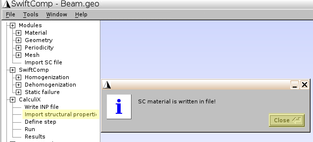
- Click
Import structural properties, to input mesh information in the INP file
- Click
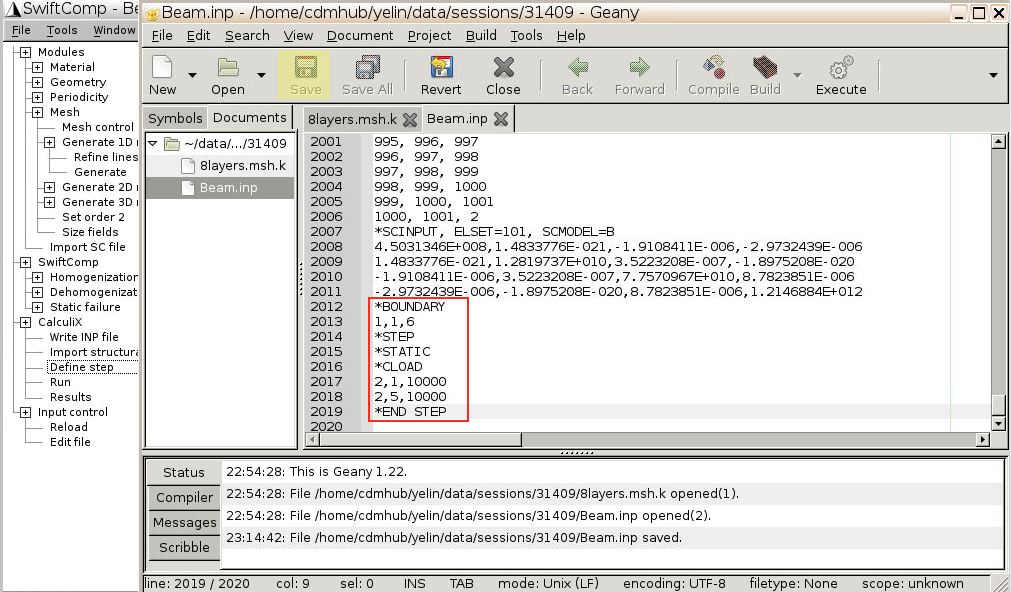
Define step, to check the input file and add boundary conditions manually

These are the {x,y,z} values for each mesh node. Notice that Node#1 and Node#2 are the two ends, x=0 and x=1000, while other nodes are increasing by step 1 since the size factor is 1.
*BOUNDARY
1,1,6
*STEP
*STATIC
*CLOAD
2,1,10000
2,5,10000
*END STEP
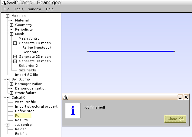
- Click
Save, close Geany editor, clickRun.
- If you’re not familiar with CalculiX, the commands you just input have the following meanings:
-
*BOUNDARY
1,1,6
1,_,_means Node#1 (x=0)
_,1,6means fixed degree of freedom 1 through 6.
Degree of freedom 1,2,3: translation in x,y,z direction;
Degree of freedom 4,5,6: rotation about x,yz, axis.
-
*CLOAD
2,1,10000
2,5,10000
CLOADmeans concentrated load
2,_,_means Node#2 (x=1000)
_,1,10000means degree of freedom 1 (translation in x direction), 10000N force
_,5,10000means degree of freedom 5 (rotation about y axis), 10000N∙mm moment
- For other types of boundary conditions, you may refer to CalculiX documentation.
- Detailed introduction for CalculiX commands used in Gmsh4SC package can be found in Chapter 4 of the Gmsh4SC User Manual.
-
3.5 Check results
- Click
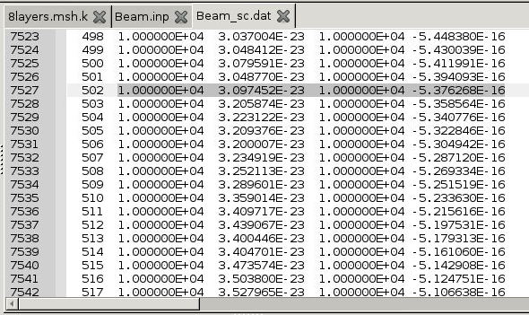
Results, and you may navigate theFilename_sc.datfile to check global responses of the beam, including Displacement ($$u_1, u_2, u_3$$), Rotation ($$\theta_1, \theta_2, \theta_3$$, Strain ($$\gamma_{11}, \kappa_1, \kappa_2, \kappa_3$$), and Stress ($$F_1, M_1, M_2, M_3$$) at nodes (x=0 through 1000) and at Gauss points.
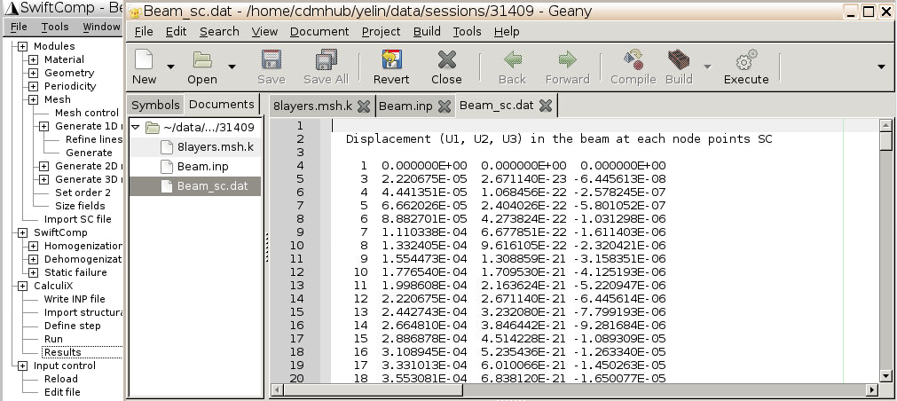
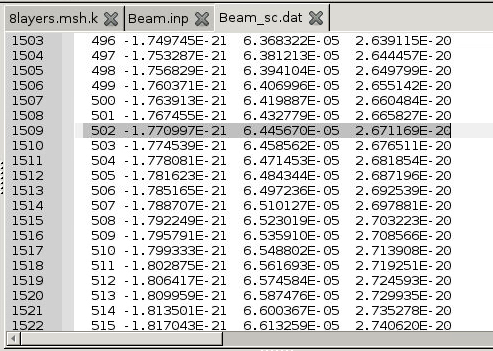
- Now you can find the global responses at each position of the beam (e.g., x = 500 mm) referring to the Node number (e.g., Node#502).

- At x = 500 mm (Node#502), the beam global responses are found to be:
$$u_1$$=1.110338E-02, $$u_2$$=6.677899E-18(=0), $$u_3$$=-1.611413E-02
$$\theta_1$$=-1.770997E-21(=0), $$\theta_2$$=6.445670E-05, $$\theta_3$$=2.671169E-20(=0),
$$\gamma_{11}$$=2.220675E-05, $$\kappa_1$$=-3.542017E-24(=0), $$\kappa_2$$=1.289142E-07, $$\kappa_3$$=5.342389E-23(=0),
$$F_1$$=1.000000E+04, $$M_1$$=3.097452E-23(=0), $$M_2$$=1.000000E+04, $$M_3$$=-5.376268E-16(=0)


- It’s more convenient to download the
Filename_sc.datfile on your local computer and search for these values. See section 2.3 of this wiki page for download instructions.
4. Dehomogenization: Local Stress Distribution
With the strain at each node given by CalculiX results, for a specific node (e.g., Node#502 at x=500 mm), we can check the local stresses in the 8 lamina layers.
4.1 Reopen microstructure geometry file
- Click
File–Open, and choose thethe_8-layer_laminate_file.geo

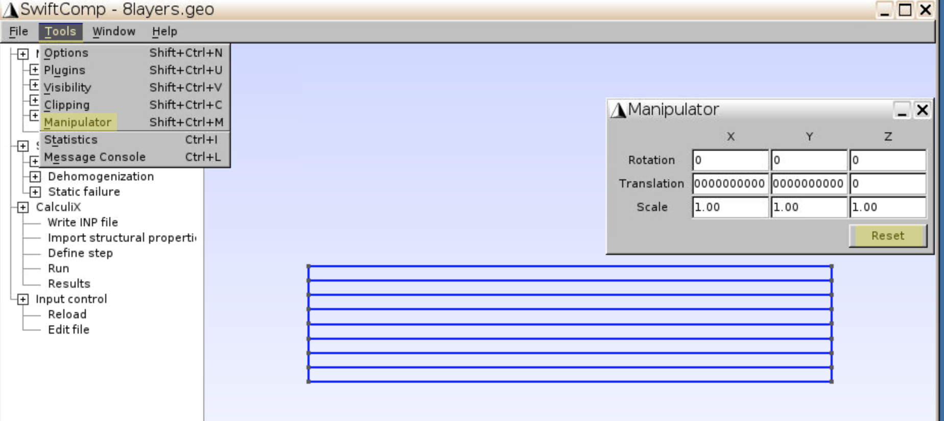
- If the 8 layer laminate geometry does not appear on the screen, it is possible that it’s outside the current view. You may bring it back by clicking
Tools–Manipulator–Reset
4.2 Dehomogenization
- Click
SwiftComp–Dehomogenization–Beam Model - Input displacement (v1, v2, v3) and strain (e11, k1, k2, k3) for Node#502. (values are given in section 3.5)

- Click
Save–Run, the results are shown on the screen with color bars. You may check the displacement, strain and stress results in thePost-processingpanel.

- Stress $$\sigma_{11}$$ of each layer is given in the following figure.

- Numerical results can be found in
filenameVIEW.msh. For example, the $$\sigma_{11}$$ results are given for each node.

4.3 Check results along a line (optional)
- To get the stress values $$\sigma_{11}$$ along the cross section (e.g., x=0, y varies from -20 to +20), you may use the CutGrid plugin.
- Click on the triangle beside S11, then click
Plugin. - Select
CutGrid,View[10](S11), and inputX0 = 0, Y0 = -20, Z0 = 0andX1 = 0, Y1 = 20, Z1 = 0. X2 Y2 Z2 can be any number as we only need two points to define a line. - NumPointsU =
100which is the number of points from {X0, Y0, Z0} to {X1, Y1, Z1}. - NumPointsV =
1which is the number of points from {X0, Y0, Z0} to {X2, Y2, Z2}. - Position of these three points are labeled on the geometry
- Click on the triangle beside S11, then click
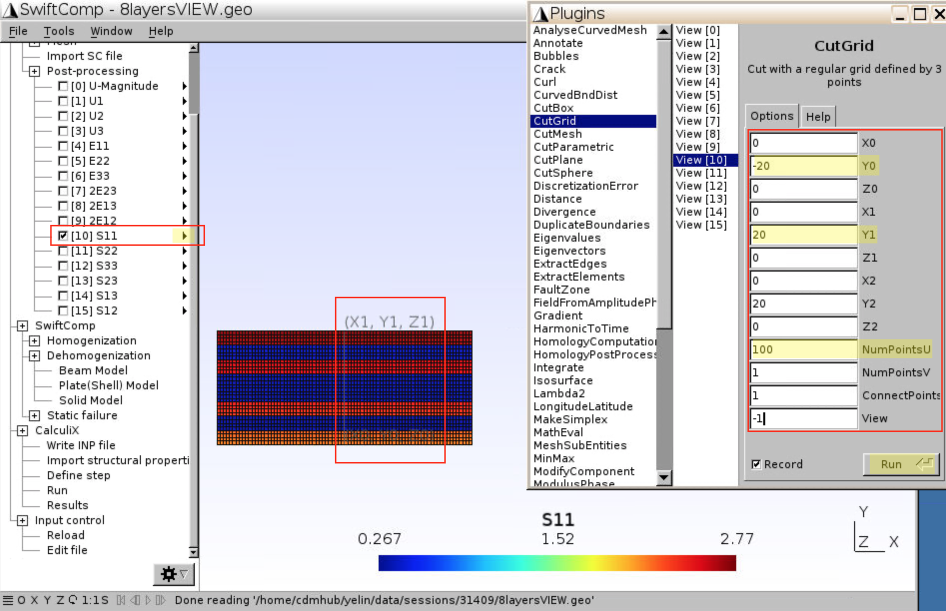
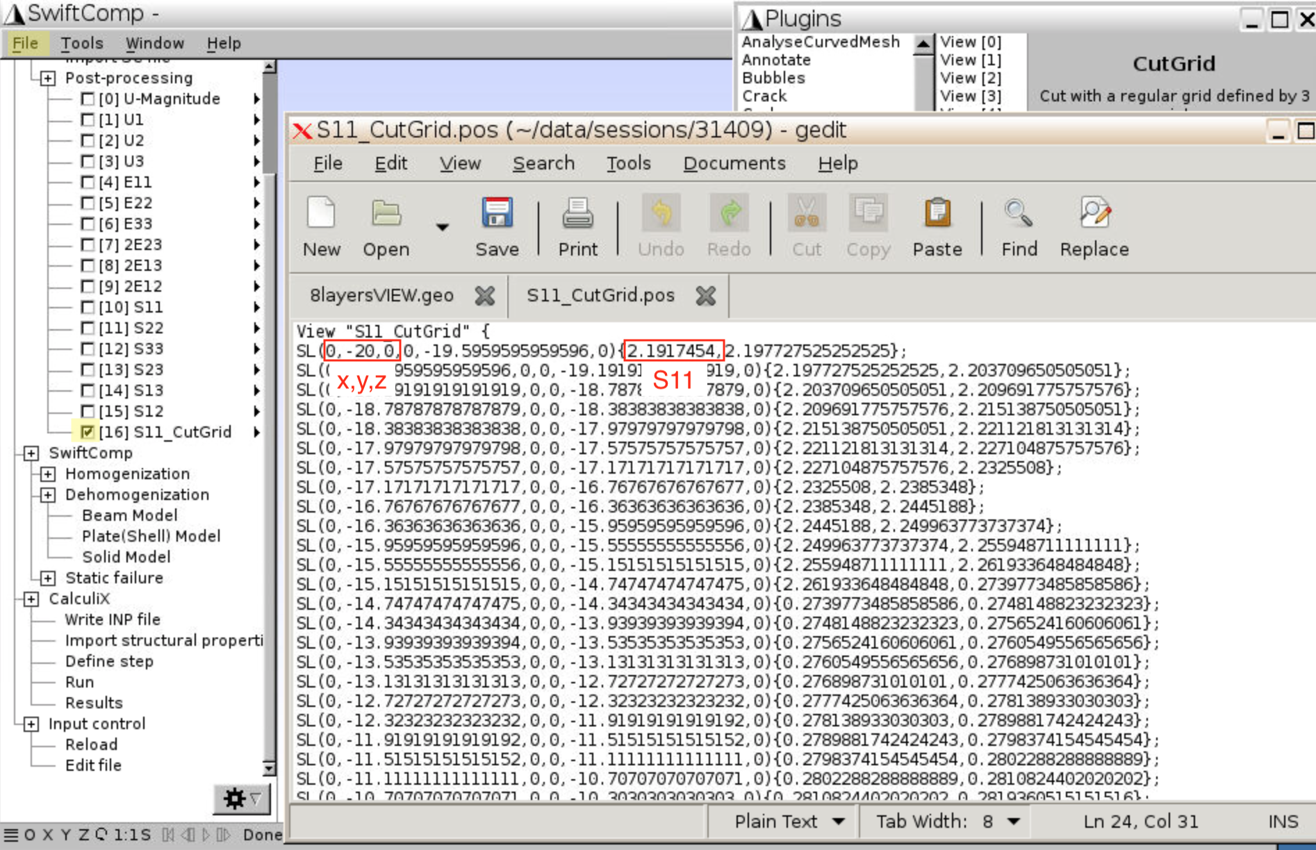
- Click
Run, and a new view will appear that only contains S11 along x=0, y= -20 to +20. You may export the new view by clicking the triangle –Export. Numerical results including {x,y,z} of each node and S11 values are recorded in the exported file.
References
- Xin Liu; Wenbin Yu (2017), “Gmsh4SC Tutorial #1: Analysis of a Composite Laminated Beam,” https://cdmhub.org/resources/1280.
- Gmsh documentation for geometry commands input
- Xin Liu; Wenbin Yu (2017), Gmsh4SC User Manual