Problem Description
In the tutorial Analysis of a Composite Laminated Beam, we analyzed the global behavior of the beam and stress distribution across beam thickness. Here we talk about cases where the cross section of the beam has complicated geometries, including:
- Boxed-shape cross section
- I-shape cross section
- User-defined cross section
This wiki tutorial as a supplement for Analysis of a Composite Laminated Beam will be focused on how to define a geometry that is compatible with SwiftComp – Homogenization calculation. After obtaining the effective stiffness matrix, you may follow the previous tutorial to calculate deformations along the beam and local stress distributions.
Software Used
- Gmsh4SC 2.0
- Gmsh 2.9.3 available at http://gmsh.info//bin/ to draw an arbitrary geometry
Resources for an earlier version of Gmsh4SC
- Analysis of Rectangular and I-shaped Beams:
- Gmsh4SC User Manual, Page 2-16 through 2-24.
- Analysis of a Boxed Beam:
- Tutorial and relevant files
- Companion video by Xin Liu:
- Analysis of a Double Cell Box Girder Bridge:
Solution Procedures
Case 1. Boxed-shape cross section
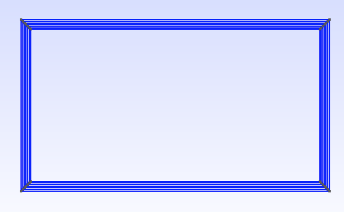
- Cross section of the beam is in the $$x_2, x_3$$ plane as shown in Fig.1.
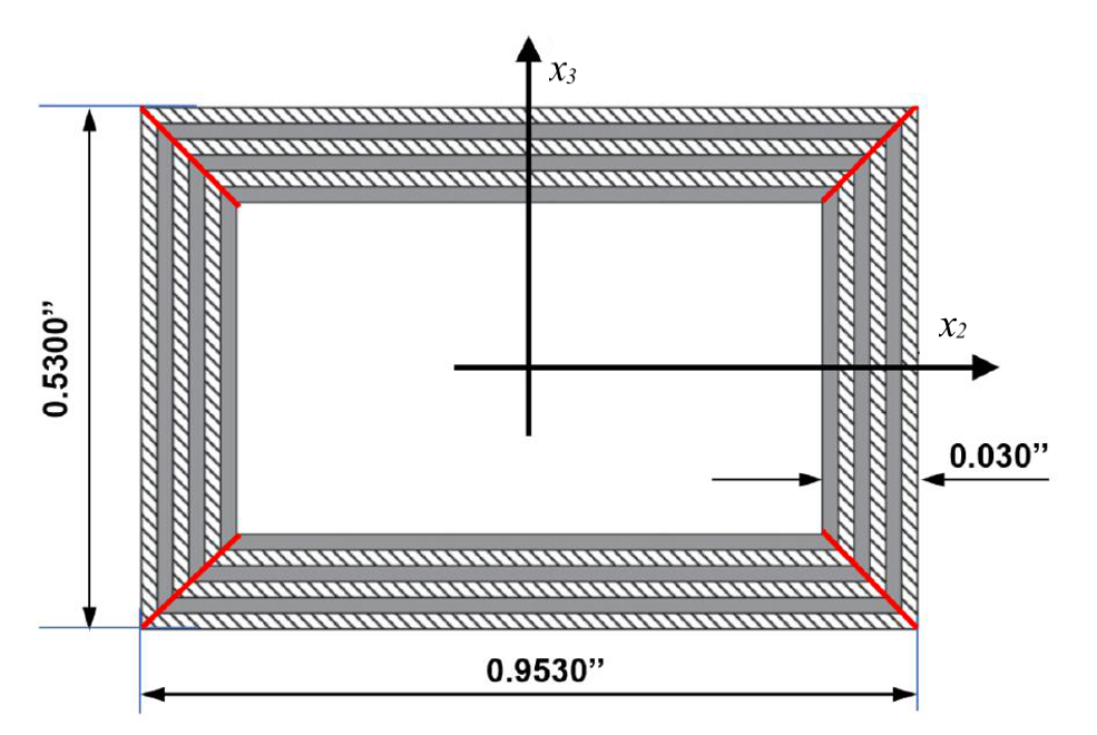
- The four walls of the box are thin composites with different layup sequences:
- Top wall: $$[-15]_6$$
- Left wall: $$[-15/15]_3$$
- Bottom wall: $$[15]_6$$
- Right wall: $$[15/-15]_3$$
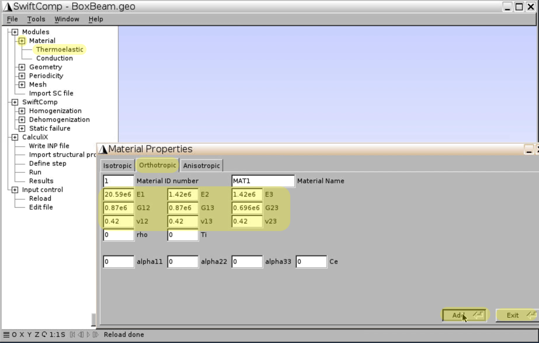
- Material properties of a lamina are given below:
- $$E_1=20.59\times10^6$$psi, $$E_2=E_3=1.420\times10^6$$psi
- $$G_{12}=G{13}=0.87\times10^6$$psi, $$G_{23}=0.696\times10^6$$psi
- $$\nu_{12}=\nu_{13}=\nu_{23}=0.42$$
- Boundary conditions of the beam:
- The beam is clamped at $$x_1 = 0$$
- The beam is subjected to 1000 lb-in bending moment about the $$x_3$$ axis at the free end (i.e., $$x_1 = 10 in$$)
First, we input material properties and laminate layup for each wall.
- Launch Gmsh4SC
- Create a new .geo file for the beam cross section
- Click
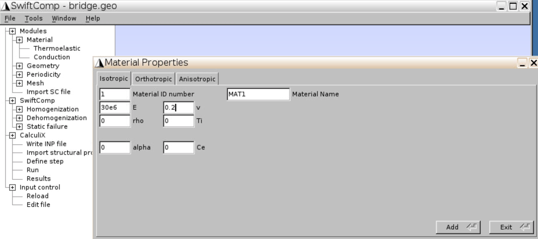
Material,Thermoelastic, chooseOrthotropicand input lamina properties, clickAdd,Exit.
- Click
Geometry,Common SG,2D,Beam sections, chooseBoxbeam section andCompositesmaterial. - Use
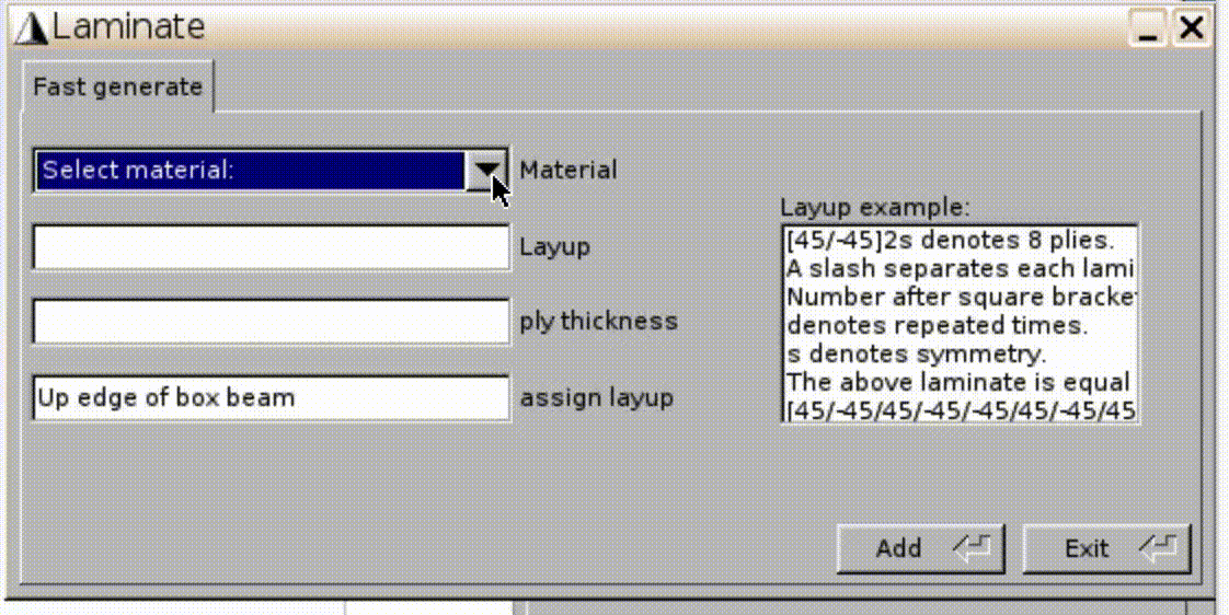
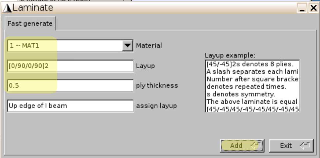
layup define,Fast generateto generate composite laminate for the four walls separately.
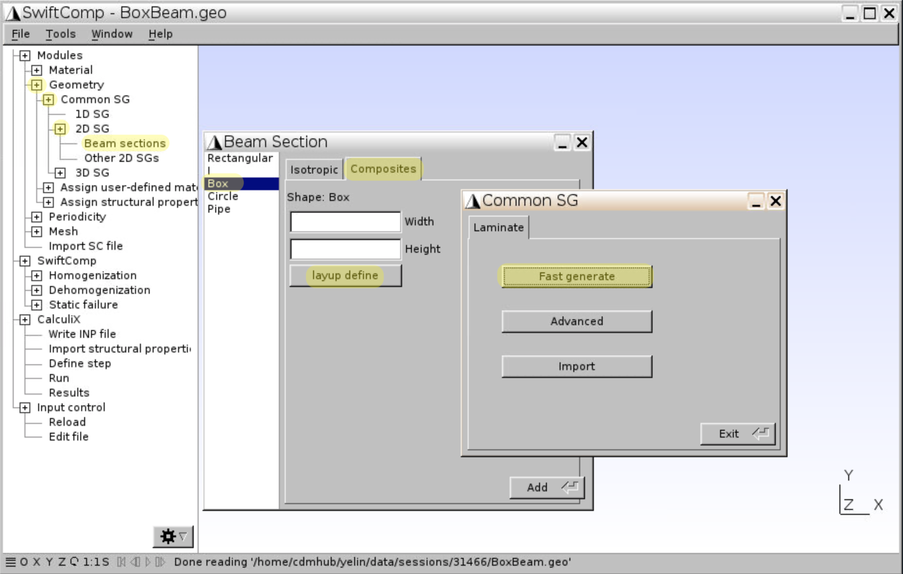
- For the upper wall, choose
1--MAT1, input[-15]6as the layup,0.005for ply thickness (0.03” for six layers), and clickAdd,Close. - Input the layups
[-15/15]3,[15]6,[15/-15]3for three other walls. ClickExit.
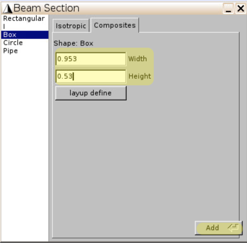
- Input Width =
0.953, Height =0.53for the boxed beam section, clickAdd. The boxed cross section will show up on screen.
- Click
Mesh,Mesh control, selectRecombine all triangular meshes(which will decrease the number of elements), and input0.5for Element size factor.

- Click
Mesh,Set order 2. (This will affect results of homogenized properties of the boxed beam section.)

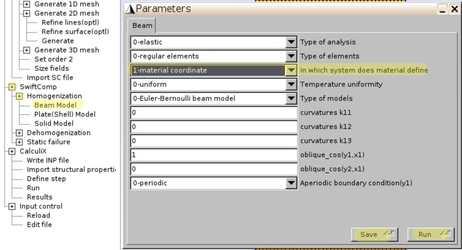
- Click
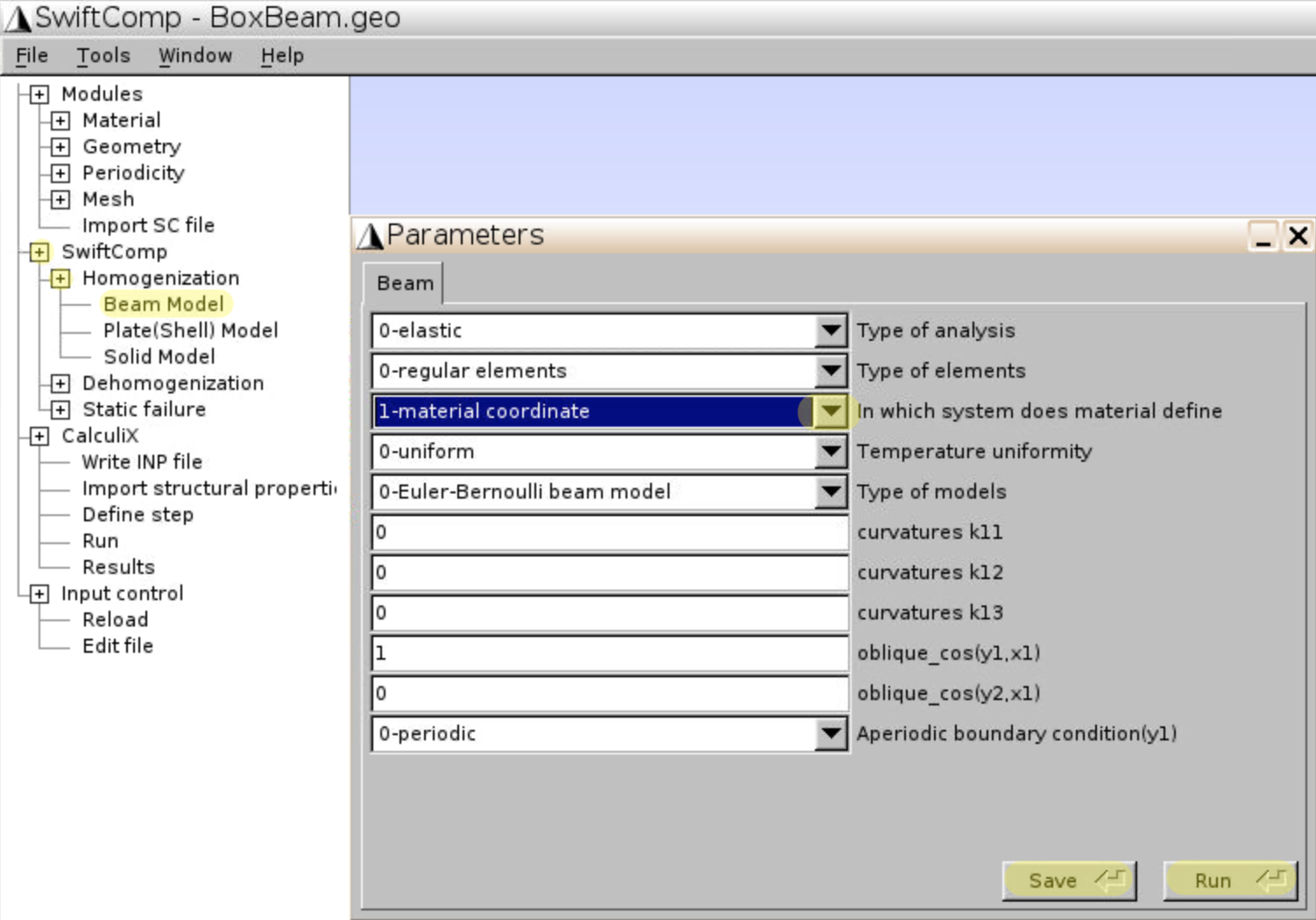
SwiftComp,Homogenization,Beam Model, choosematerial coordinateas the coordinate system, and clickSaveandRun.
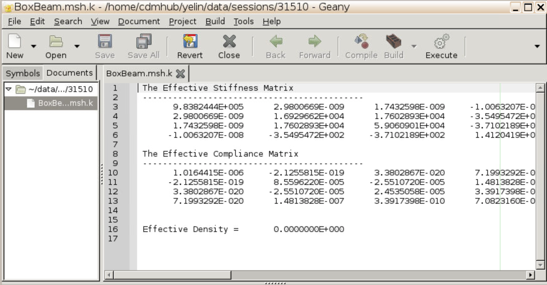
- The effective stiffness and compliance matrices are automatically stored in .msh.k file and will pop up on the screen. Feel free to download the .msh.k file to your local computer.
Analysis of the entire beam and local stress distribution follow the same procedure as in Analysis of a Composite Laminated Beam. Briefly, you’ll need to create a new .geo file, draw a line to represent the beam, assign the .msh.k file as structural property and use CalculiX to calculate displacements and rotations along the beam. In this case, the boundary conditions to be added at the end of CalculiX .inp file should be
*BOUNDARY
1,1,6
*STEP
*STATIC
*CLOAD
2,6,1000
*END STEP
where 1,1,6 means node#1 ($$x_1 = 0, x_2 = 0, x_3 = 0$$) has fixed degree of freedom 1 through 6, 2,6,1000 means node#2 ($$x_1 = 10, x_2 = 0, x_3 = 0$$) has the degree of freedom 6 (rotation about $$x_3$$ axis) of magnitude 1000 lb-in.
For a particular node, you may further check the localized stress distribution by doing dehomogenization to the .geo file for boxed beam cross section.
Case 2. I-shape cross section
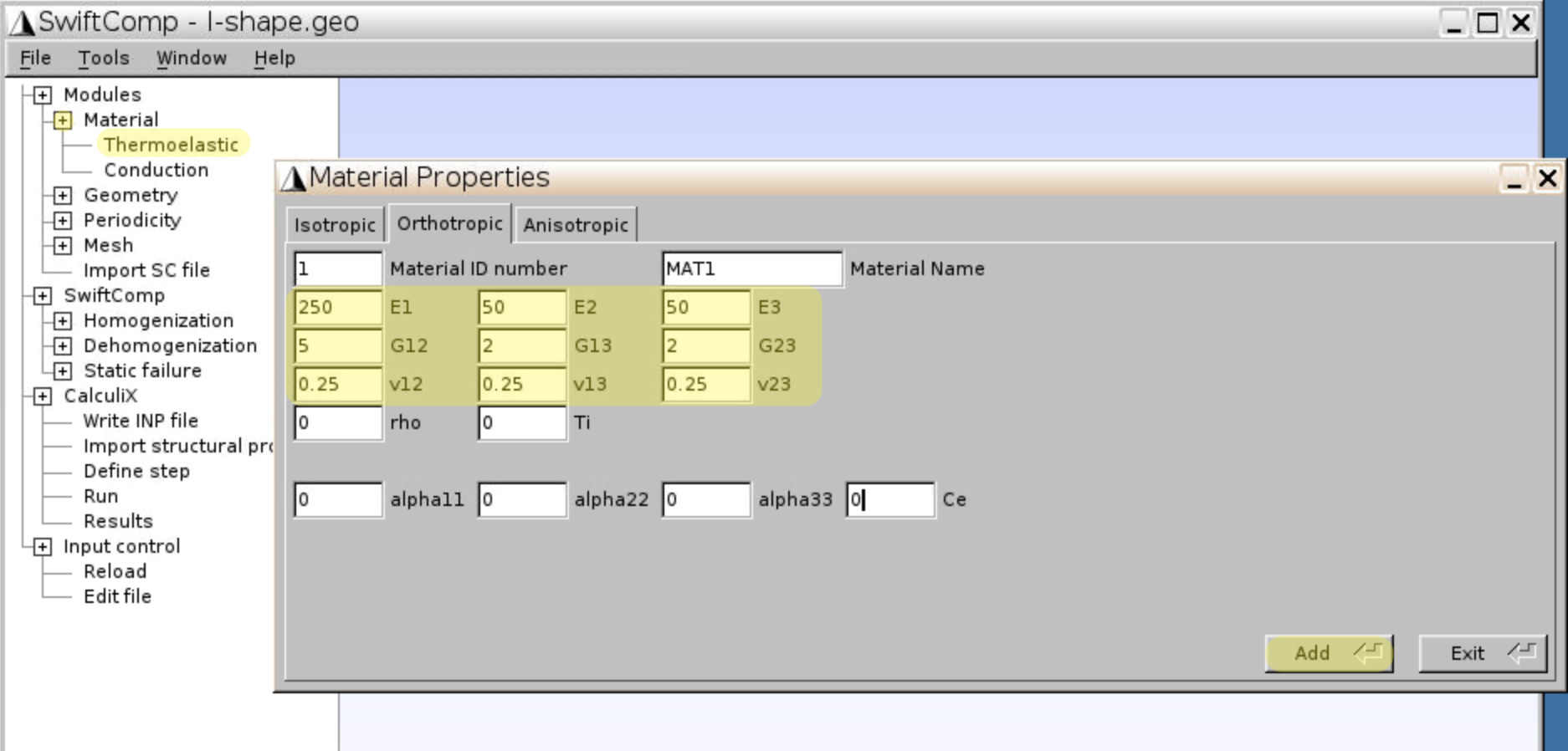
- First, input material constants: $$E_1=250$$GPa, $$E_2=E_3=50$$GPa, $$G_1=5$$GPa, $$G_2=G_3=2$$GPa, $$\nu_{12}=\nu_{13}=\nu_{23}=0.25$$ in
Material,Thermoelastic,Orthotropictab
- Click
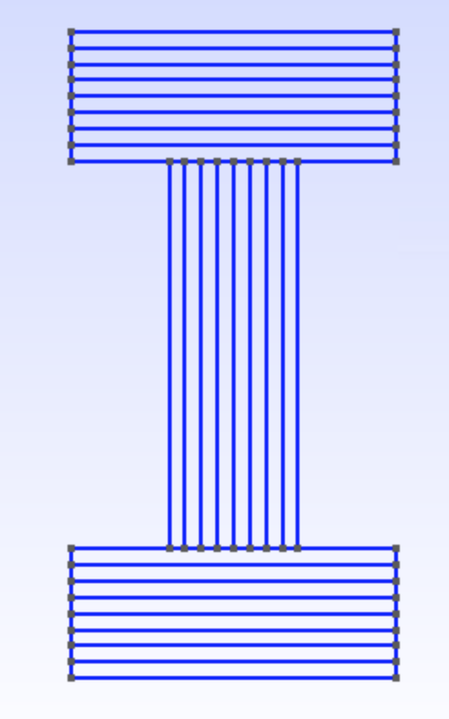
Geometry,Common SG,2D,Beam sections, chooseIbeam section andCompositesmaterial. - Input height h =
20, bottom flange width b1 =10, top flange width b2 =10.
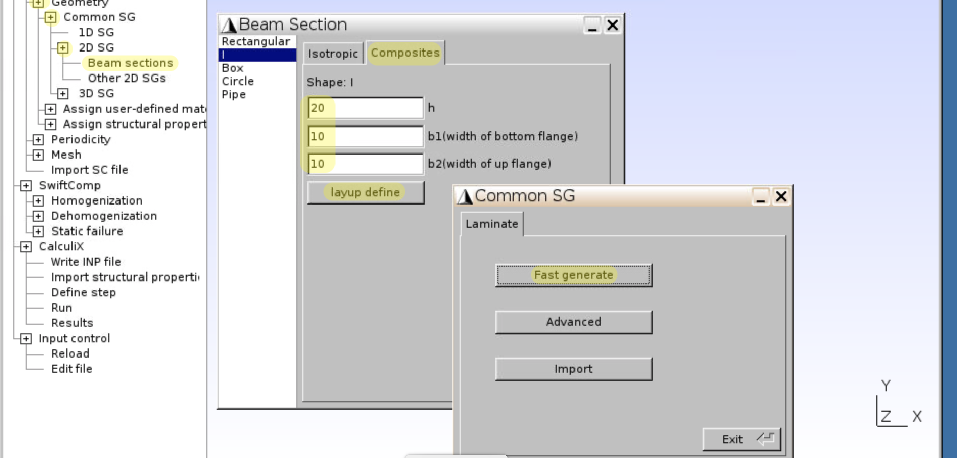
- Use
layup define,Fast generateto generate composite laminate. - Both bottom and top flange have the same layup
[0/90/0/90]2and ply thickness0.5.
- The geometry for the I-shaped beam section will pop up.
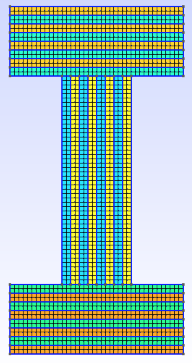
- Before generation of mesh elements, go to
Mesh,Mesh control, and selectRecombine all triangular meshesand input0.5for Element size factor.

- You will see the meshed beam section.
- Click
SwiftComp,Homogenization,Beam Model, choosematerial coordinateas the coordinate system, and clickSaveandRun.
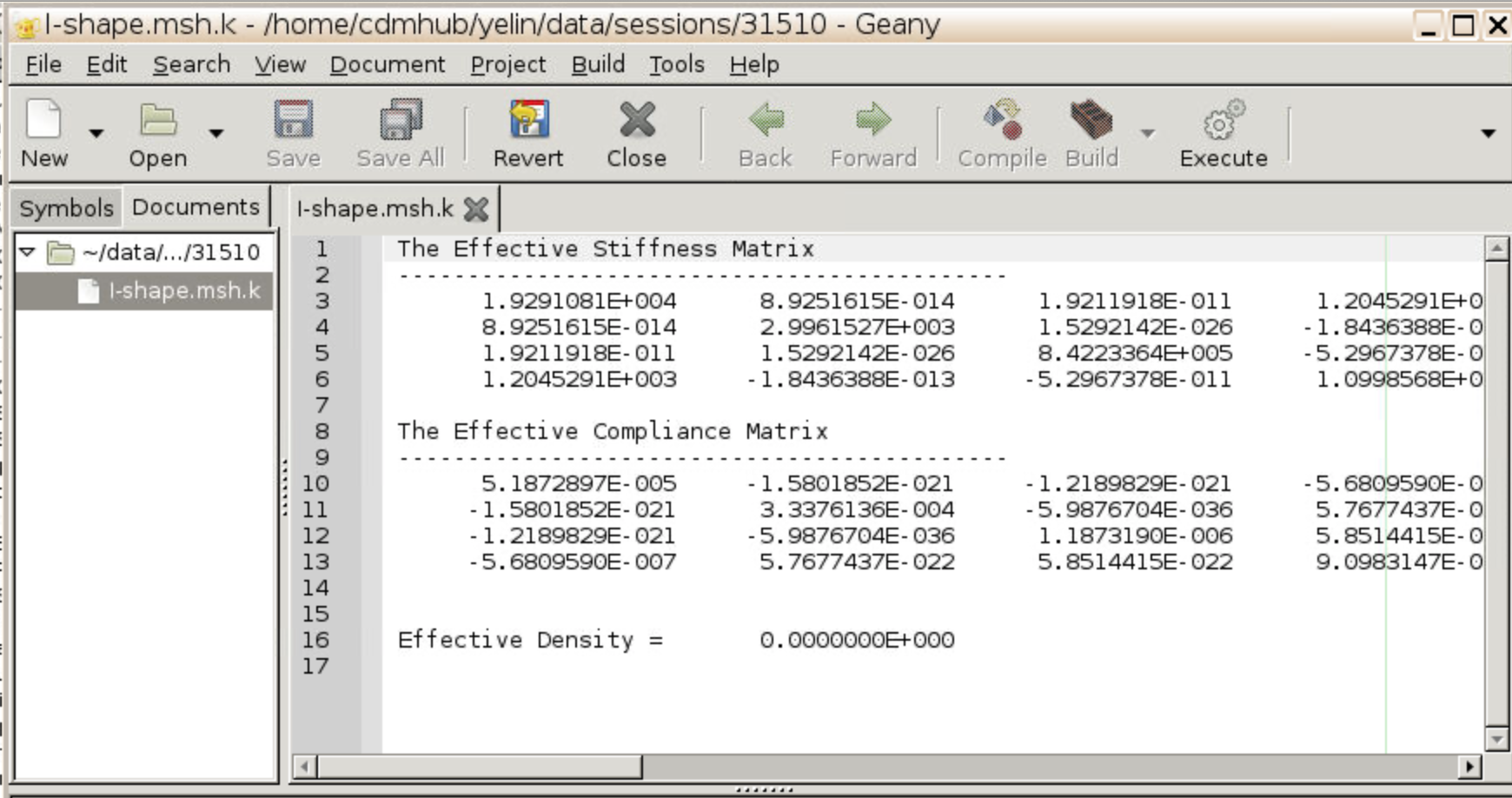
- The effective stiffness and compliance matrices are automatically stored in .msh.k file and will pop up on the screen.
Case 3. User-defined cross section
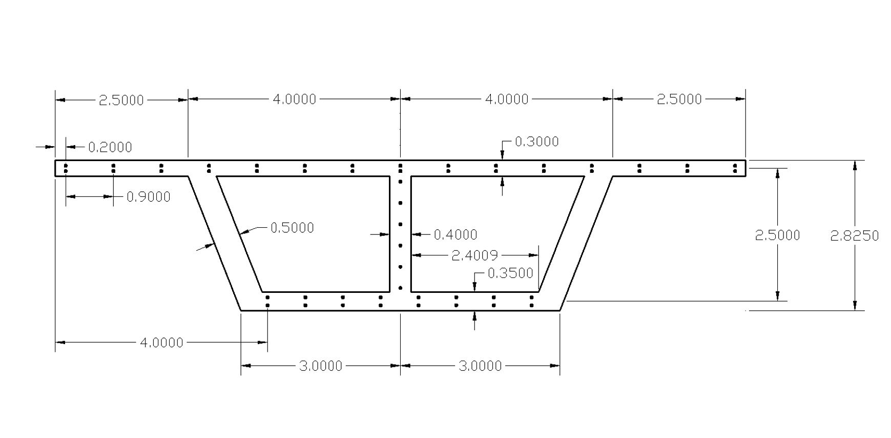
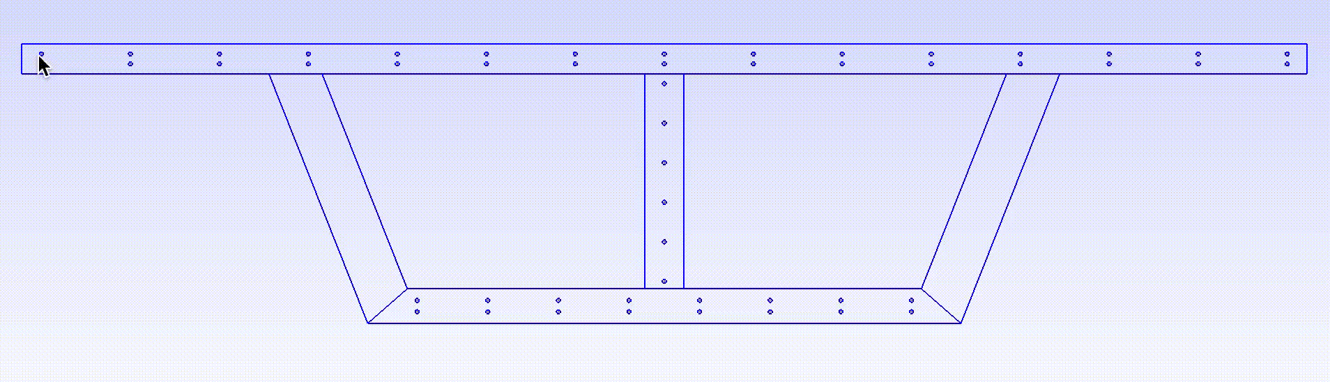
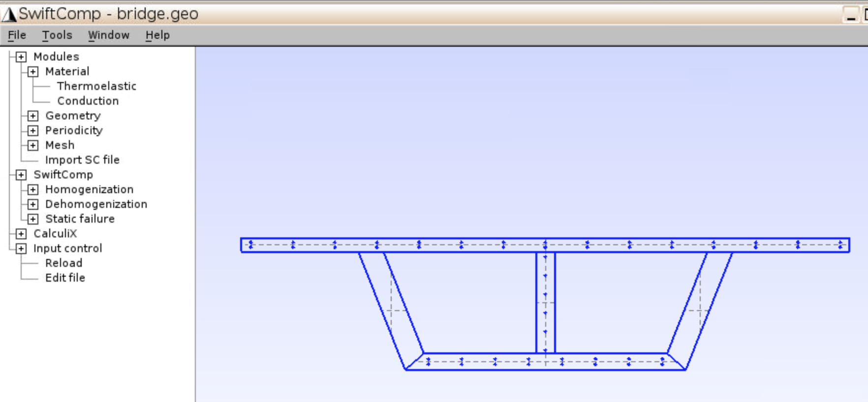
- Here, we use the cross section of a double-cell box girder bridge to demonstrate how to draw an arbitrary shape that is not included in
Common SG. The drawing of the cross section is given in Figure 19.
- The current version of SwiftComp does not have CAD function. To define a complicated geometry, it’s better to download !Gmsh on your local computer, draw the cross section and upload to cdmhub server.
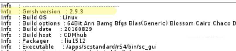
- In Message Console, you may find
Gmsh version: 2.9.3which is the version incorporated in !Gmsh4SC on cdmhub. We need to download the same version. If you use a later version of !Gmsh, the commands to define the same type of geometry will be different, and cannot be recognized by !Gmsh4SC.
- The stand alone Gmsh.exe is uploaded as a Supporting Docs of SwiftComp. Or, you may find the 2.9.3 version for your operation system here: http://gmsh.info//bin/
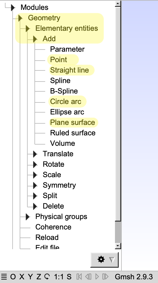
- Launch the !Gmsh on your local computer, add
Point, then useStraight lineorCircle arcto connect points, and finally createPlane surface.
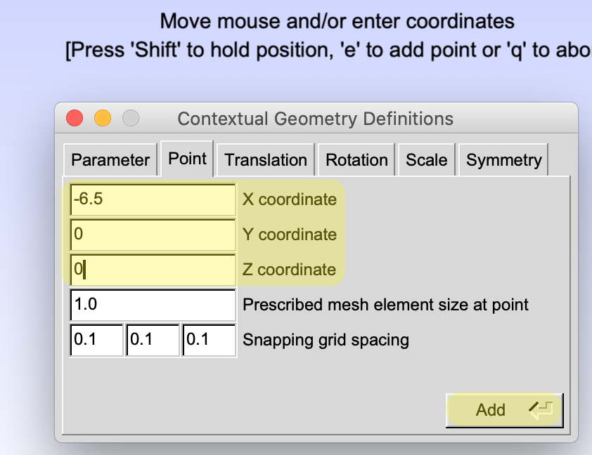
- Input the (x,y,z) values of the points, click
Add.
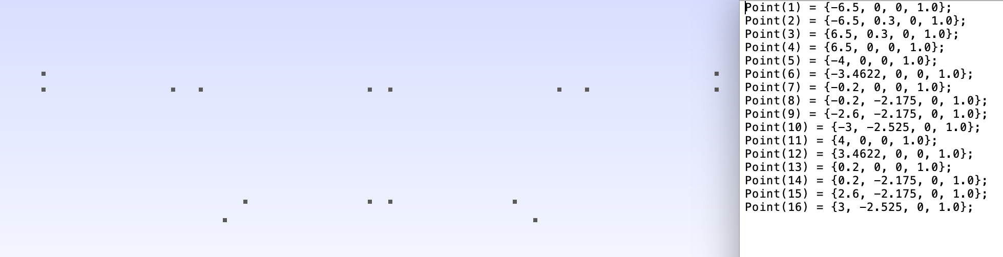
- The (x,y) values of intersections are given in Figure 23, z = 0.
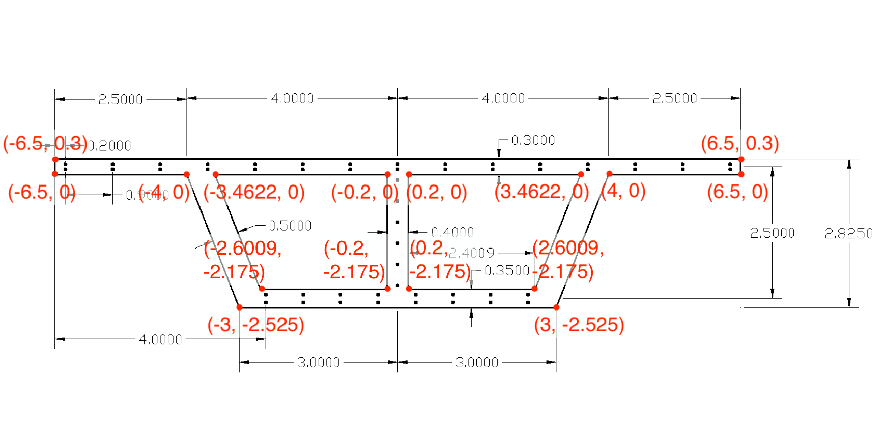
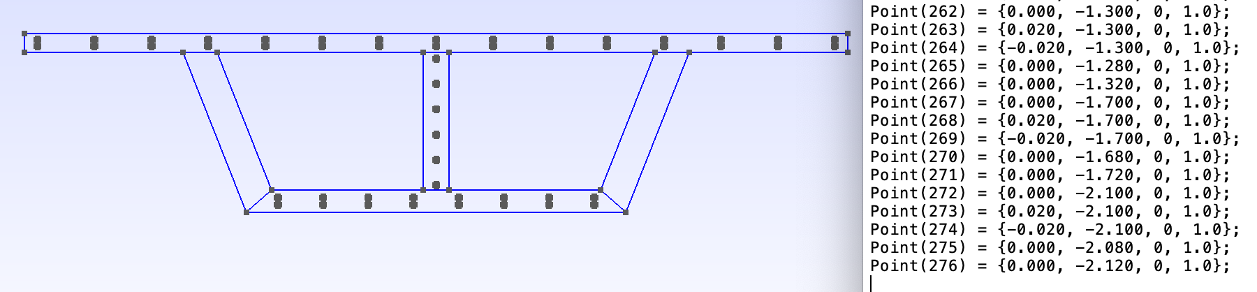
- Add the 16 points.
- Add
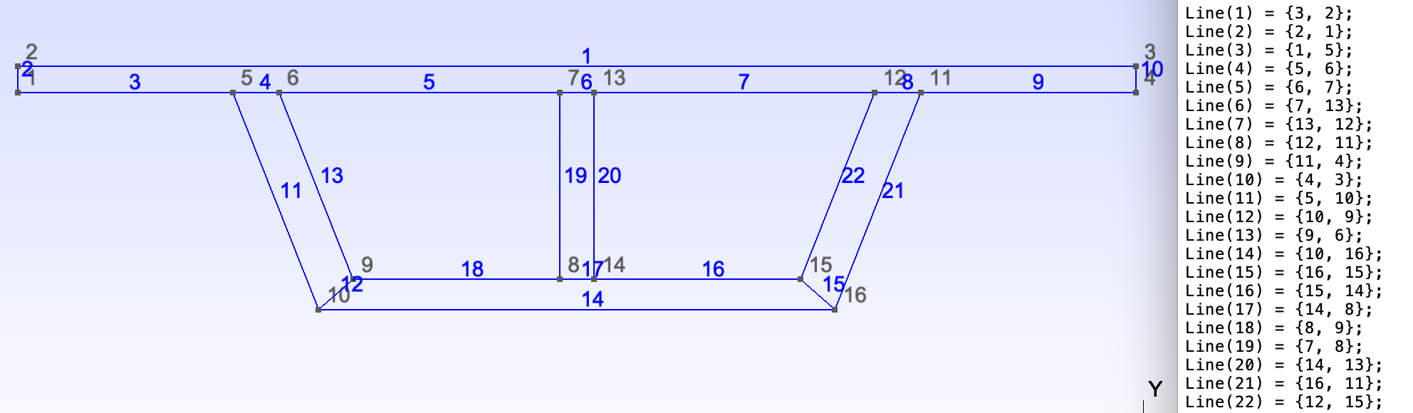
Straight line, click two points to create a line. Create the 22 lines connecting the 16 points.
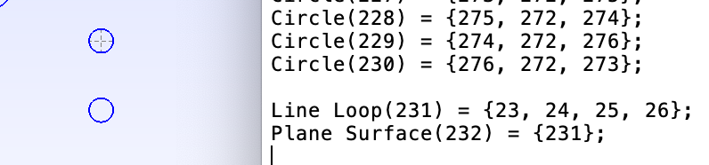
- Create 52 circular holes that represent steel cross sections. Each circle is defined by 5 points and 4 arcs:
- circle center: {x, y, z, mesh size} (z = 0, mesh size = 1)
- right edge: {x+R, y, z, mesh size} (R is radius, R=0.02)
- left edge: {x-R, y, z, mesh size}
- top edge: {x, y+R, z, mesh size}
- bottom edge: {x, y-R, z, mesh size}
- each arc is created by clicking one point on the edge – circle center – the adjacent point on the edge.
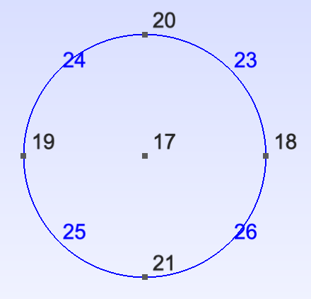
- For example, the points and arcs of the circle in the figure are given as:
Point(17) = {-2.500, -2.292, 0, 1.0};
Point(18) = {-2.480, -2.292, 0, 1.0};
Point(19) = {-2.520, -2.292, 0, 1.0};
Point(20) = {-2.500, -2.272, 0, 1.0};
Point(21) = {-2.500, -2.312, 0, 1.0};
Circle(23) = {18, 17, 20};
Circle(24) = {20, 17, 19};
Circle(25) = {19, 17, 21};
Circle(26) = {21, 17, 18};
- Create the other circular holes. Figure 27 shows the location of circle centers on the right side of the cross section. The left side is symmetric.

- The values of circle centers given in Figure 27 are calculated assuming that circular holes are evenly distributed. (e.g., vertical space = 0.35/3 for holes on the lower bar.)
- Feel free to automatically generate commands by coding or Excel functions. You can open .geo file by text editor, or click
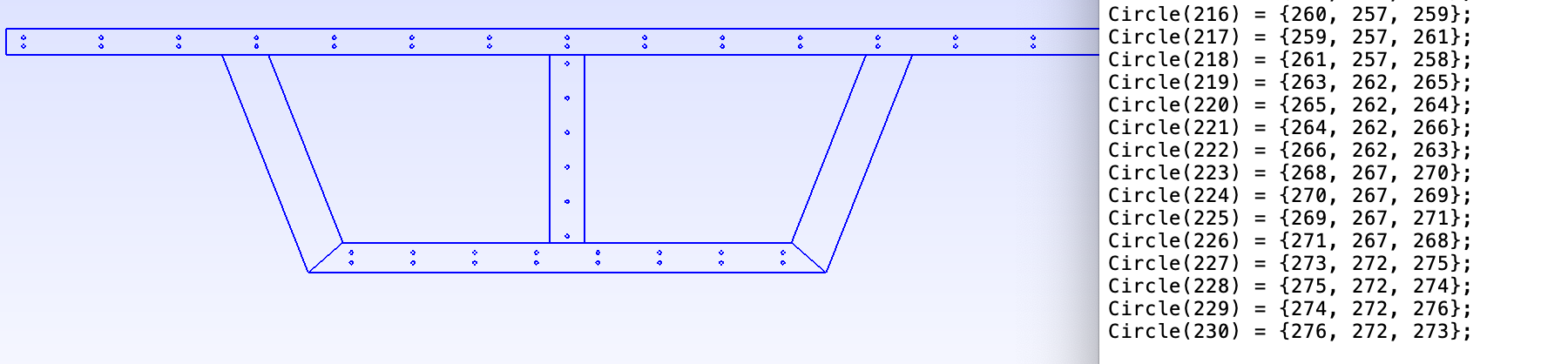
Geometry,Edit fileto paste the commands, and clickGeometry,Reloadfor the new points and arcs to show up. - All 52 circular holes are described by 260 points (Point #17 ~ Point #276) and 208 arcs (Circle #23 ~ Circle #230).
- Create
Plane surfacefor each circular hole by clicking the arc boundaries, and presse. Each surface is represented by crossed grey dashed lines.
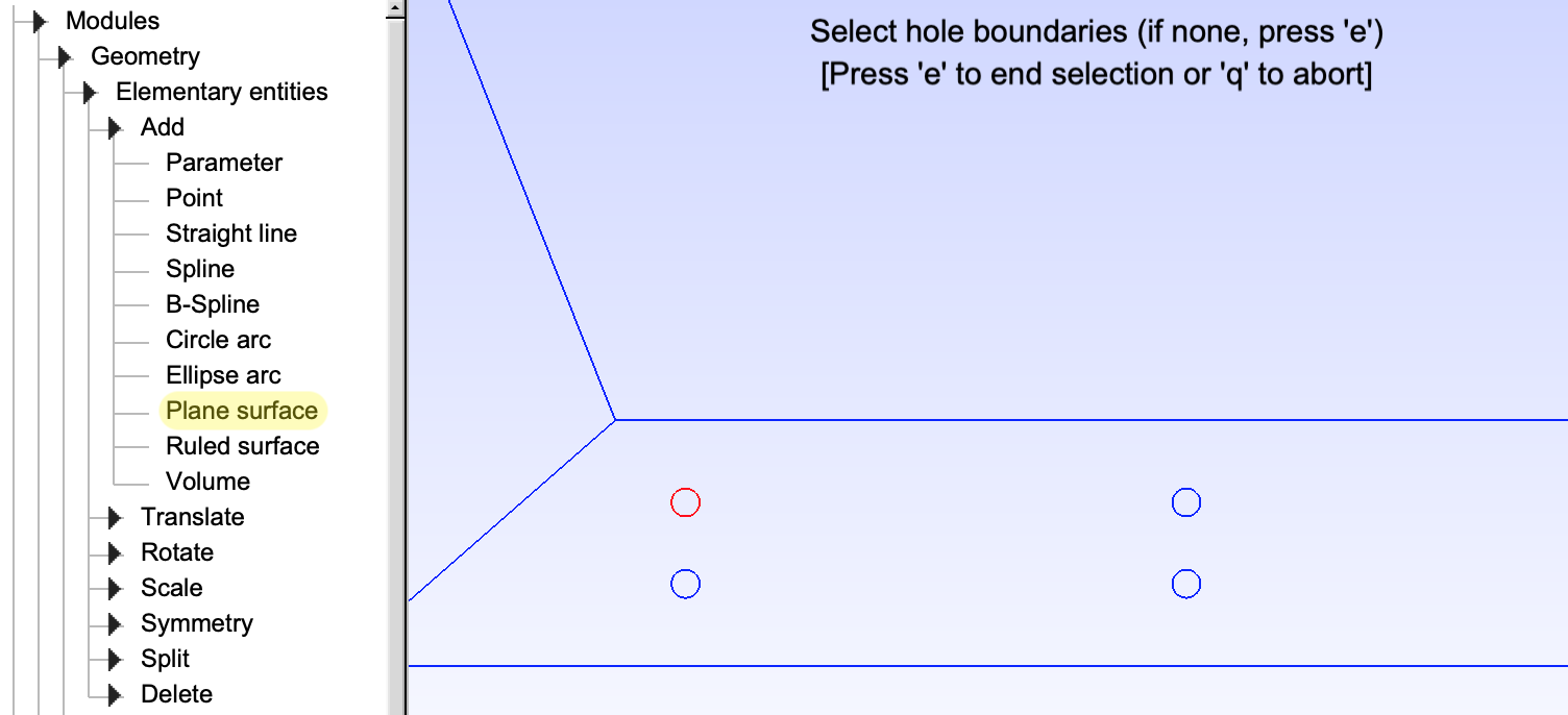
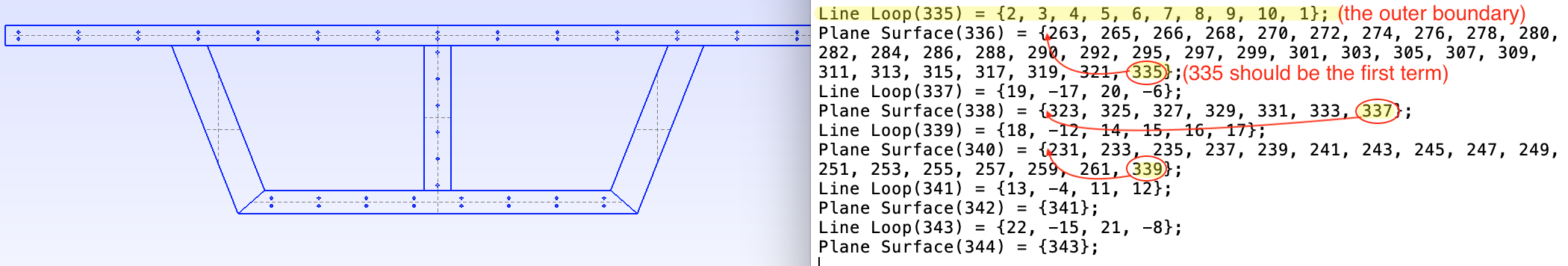
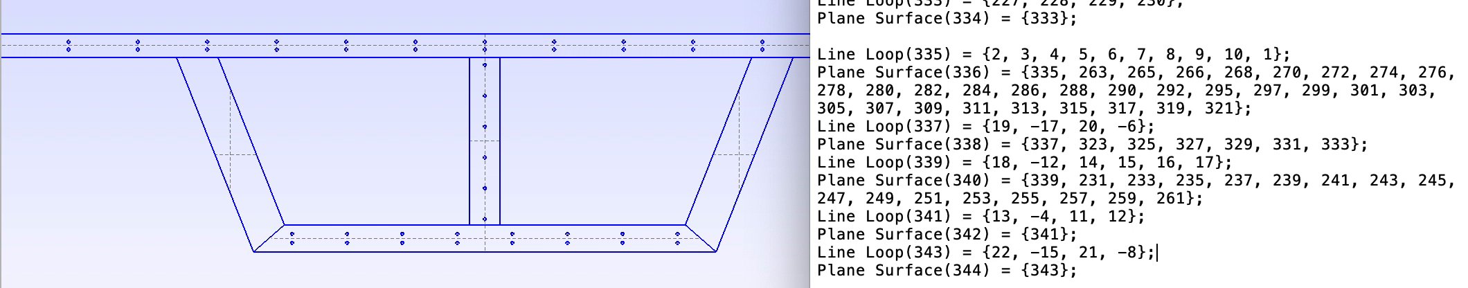
- These circular holes will be assigned with material properties of steel. The rest of the cross section will be assigned with concrete properties. Now create the surfaces for concrete by clicking
Plane surface, clicking the contour including outer loop and holes to be excluded, then presse.
- Click
Edit fileor open the .geo file in a text editor to double check that the command to create surfaces start with outer line loop followed by inner line loops, i.e., the command should bePlane Surface(#) = {outer loop # for the rectangular bar, inner loop # for holes, ...};Sometimes !Gmsh will arrange the numbers in ascending order, which will cause failure of calculation.
- The cross section is finished. Now we launch Gmsh4SC, create a new .geo file, input material properties.

- Upload the cross section drawing file that you just created to the cloud.
- Click
Input control,Edit file, open the uploaded .geo file, copy all commands and paste into the current .geo after// Material name: 2starting a new line.

- Click
Reload. The cross section of the bridge should appear. If the cross section does not appear or the session terminates, it means the commands contain error. Reopen the .geo file with your local !Gmsh and check if there’s error in message console.
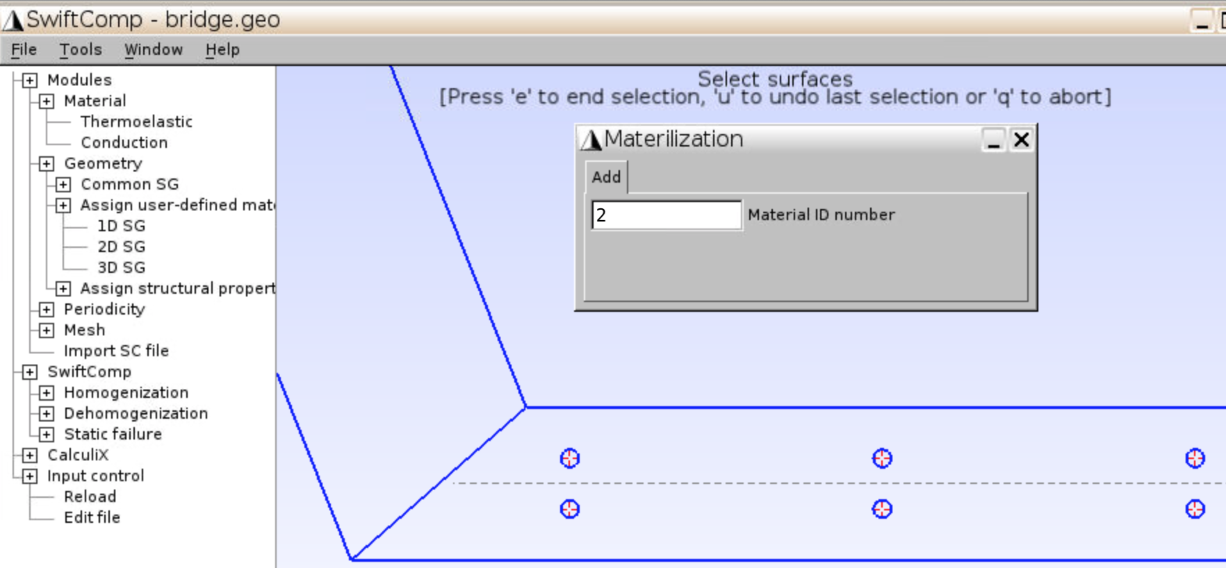
- Click
Geometry,Assign user-defined material,2D SG. With Material ID1, click the 5 pairs of grey lines (representing surfaces) for the concrete parts, the selected surfaces are labeled as red lines. Presseafter 5 surfaces are selected.
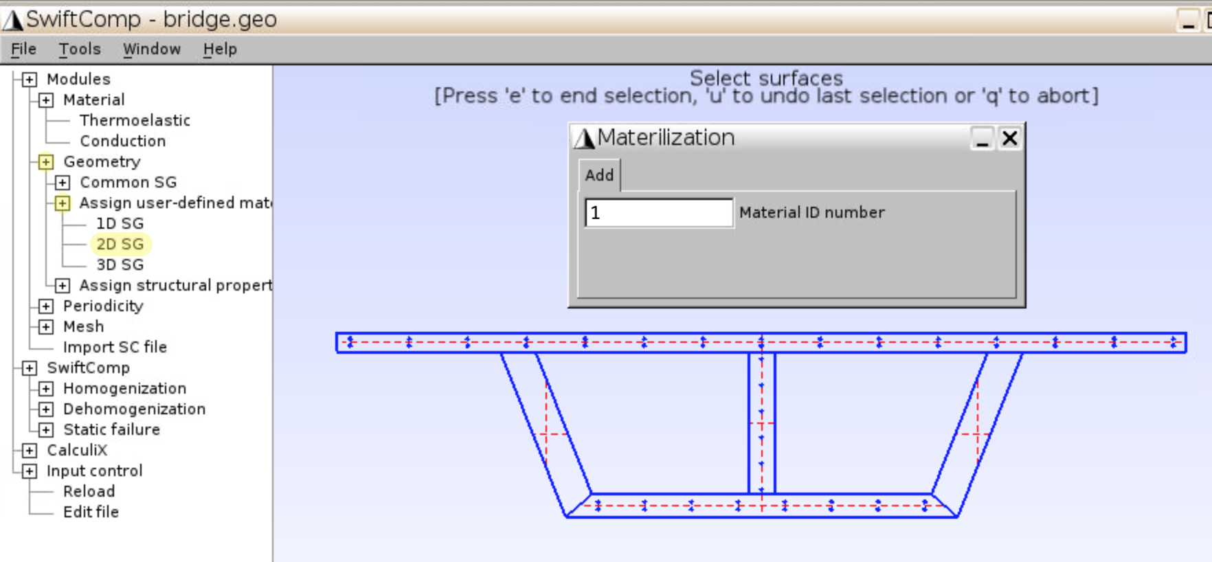
- Change the Material ID to
2, click all 52 circular surfaces so that they’re assigned with steel properties, presseandu.
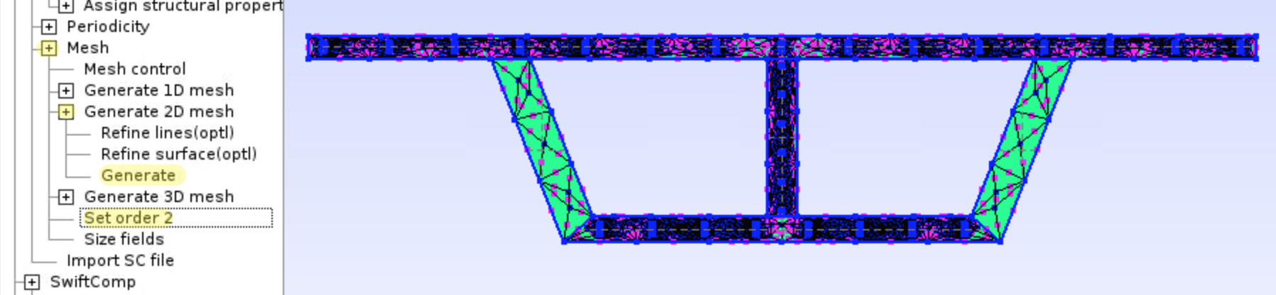
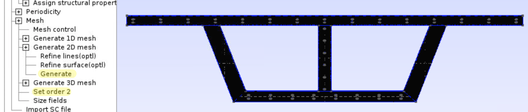
- Click
Mesh,Generate 2D mesh,Generate, andSet order 2.
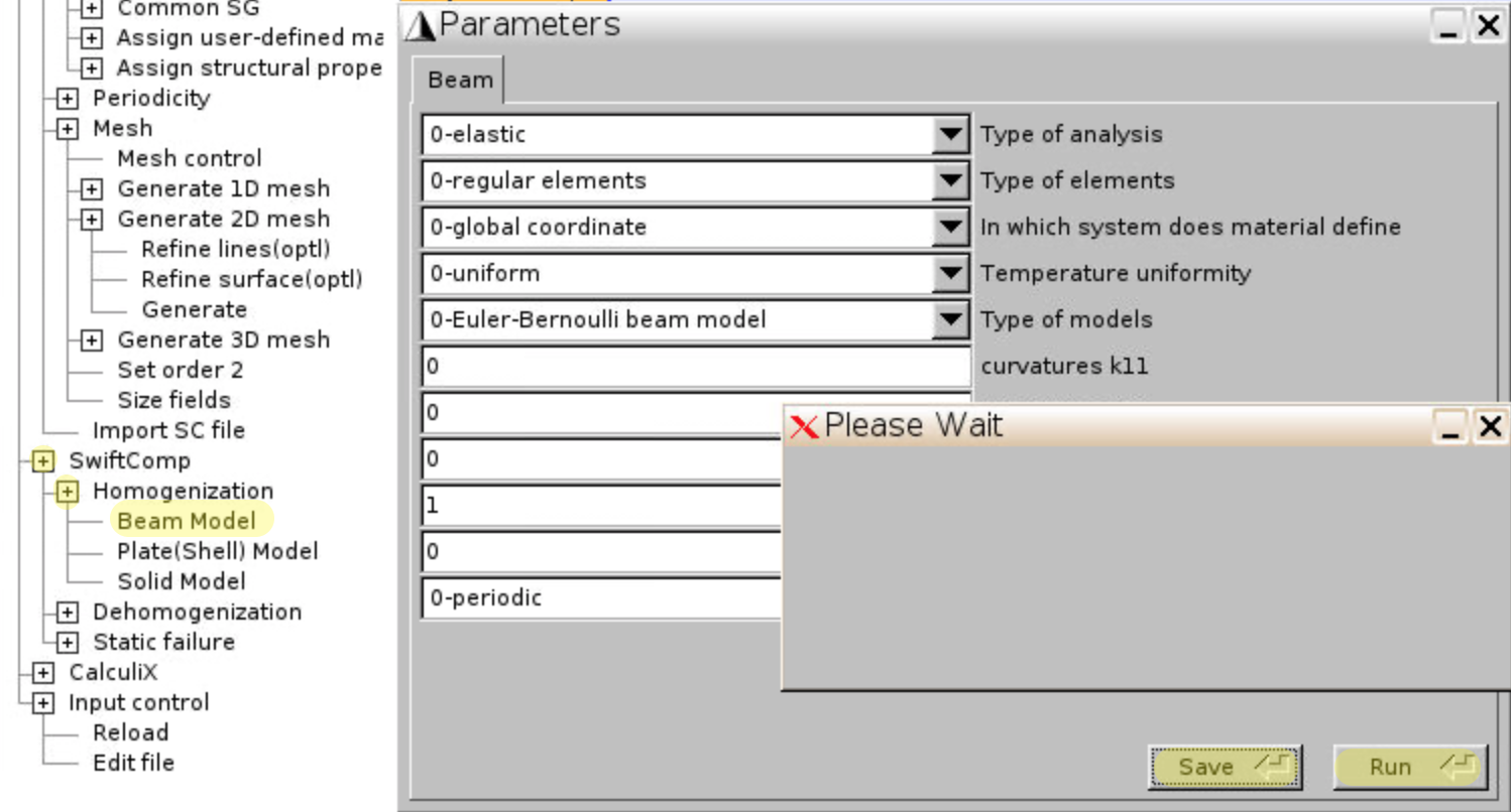
- Click
SwiftComp,Homogenization,Beam Model, keep the default setting, clickSave,Run.
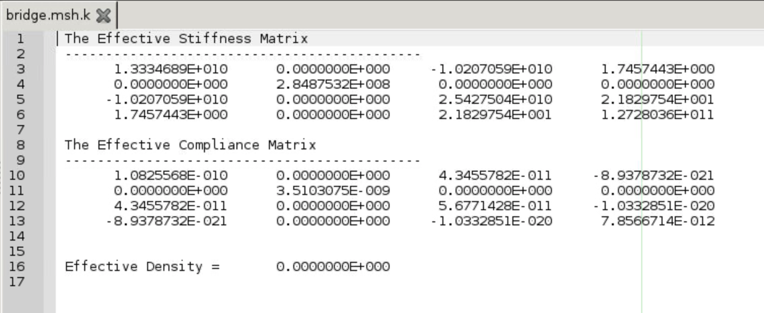
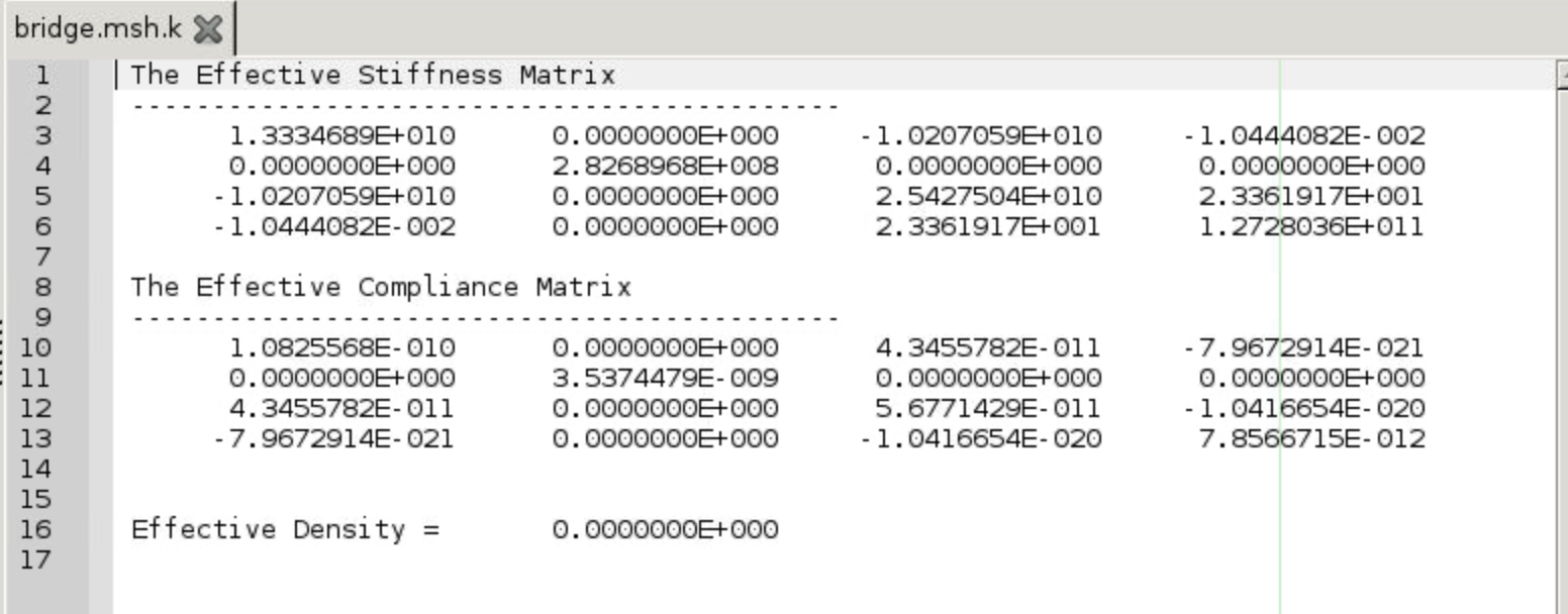
- Figure 44 shows the homogenization results (i.e., effective stiffness matrix of the SG).
- Follow the same procedure as in Analysis of a Composite Laminated Beam to calculate the deformation of the entire bridge. Boundary conditions to be added at the end of .inp file are
*BOUNDARY
1,1,6
*STEP
*STATIC
*CLOAD
2,5,5000000
*END STEP
which means the bridge is fixed at x = 0 (node#1), and subjected to a 5000 kN-m moment in y-direction at x = 150m (node#2). Check the displacement and rotation at a specific node in _sc.dat file. This will be used as the input for dehomogenization.
- Reopen the .geo file for cross section of bridge. Before dehomogenization, we need to apply finer meshing in order to capture the localized stress distribution along thickness. First click
Edit fileand delete previous mesh (lines starting fromMesh.Points=1;)

- Click
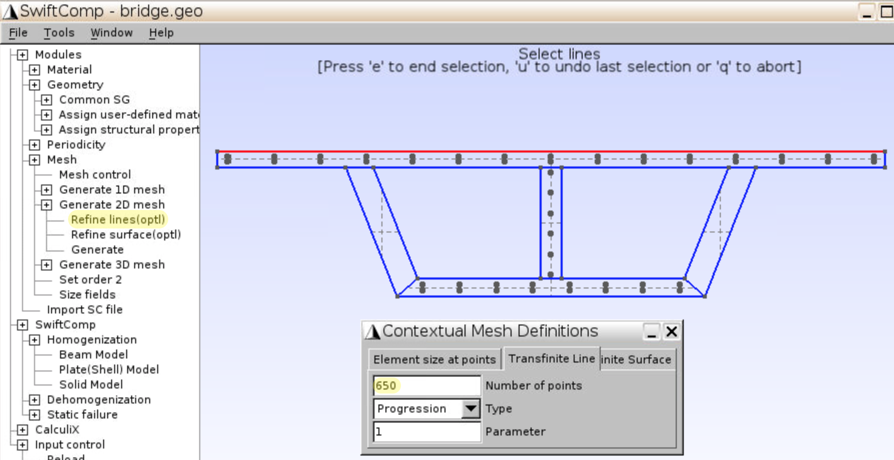
Mesh,Generate 2D mesh,Refine lines, input Number of points =650, click the upper boundary of the bridge, presse.
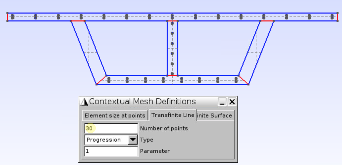
- Input Number of points =
30, click the short lines as shown in Figure 47, presse.
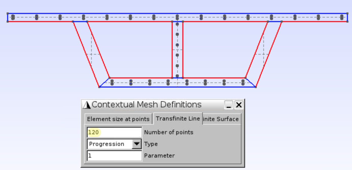
- Input Number of points =
120, click the vertical lines and separated horizontal lines as shown in Figure 48, presse.
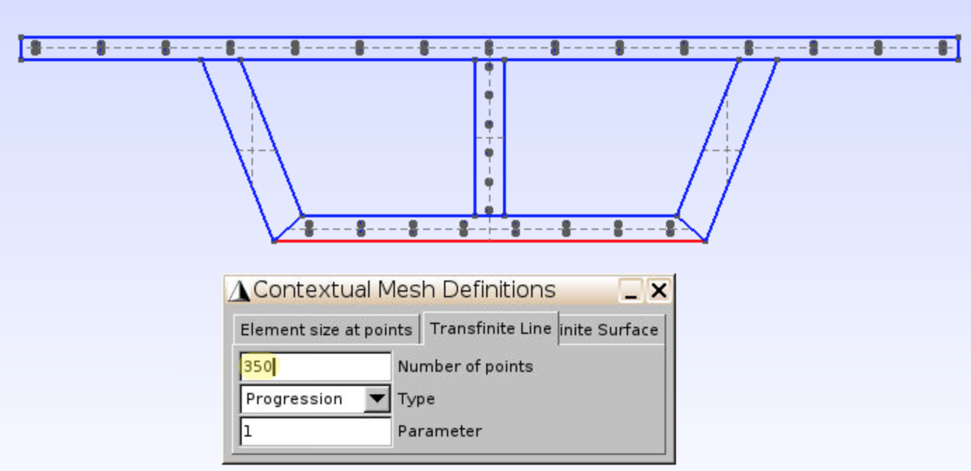
- Input Number of points =
350, click the lower boundary, presse,u.
- You may also refine the mesh of circles using more than 3 points for each arc, which will help in order to check the stress distribution inside the holes.
- Click
Generate 2D mesh,Generate, andSet order 2. It takes 20-30 seconds to see the meshed geometry.

- Double check the effective stiffness matrix given by
Homogenizationafter refined meshing is the same as the results of coarse meshing.
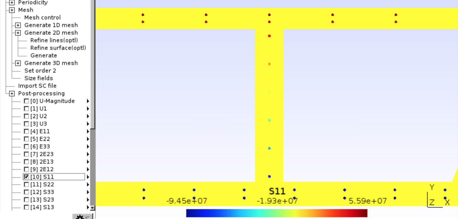
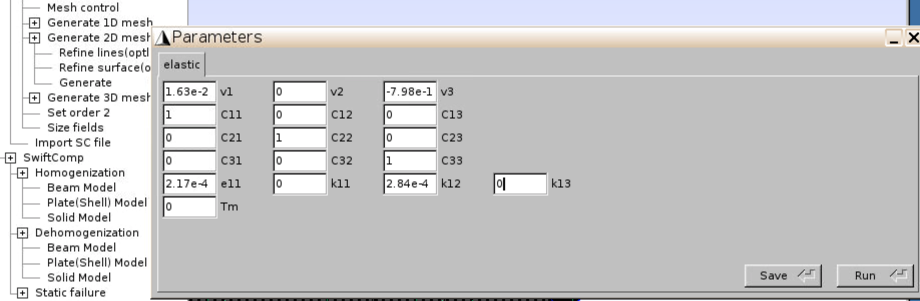
- Click
SwiftComp,Dehomogenization,Beam Model, and input the v1, v2, v3, e11, k11, k12, k13 values found in _sc.dat file (the output of CalculiX). The values in Figure 53 are for Node#77 (x=75m). ClickSave,Run.
- Check the strain and stress distribution.
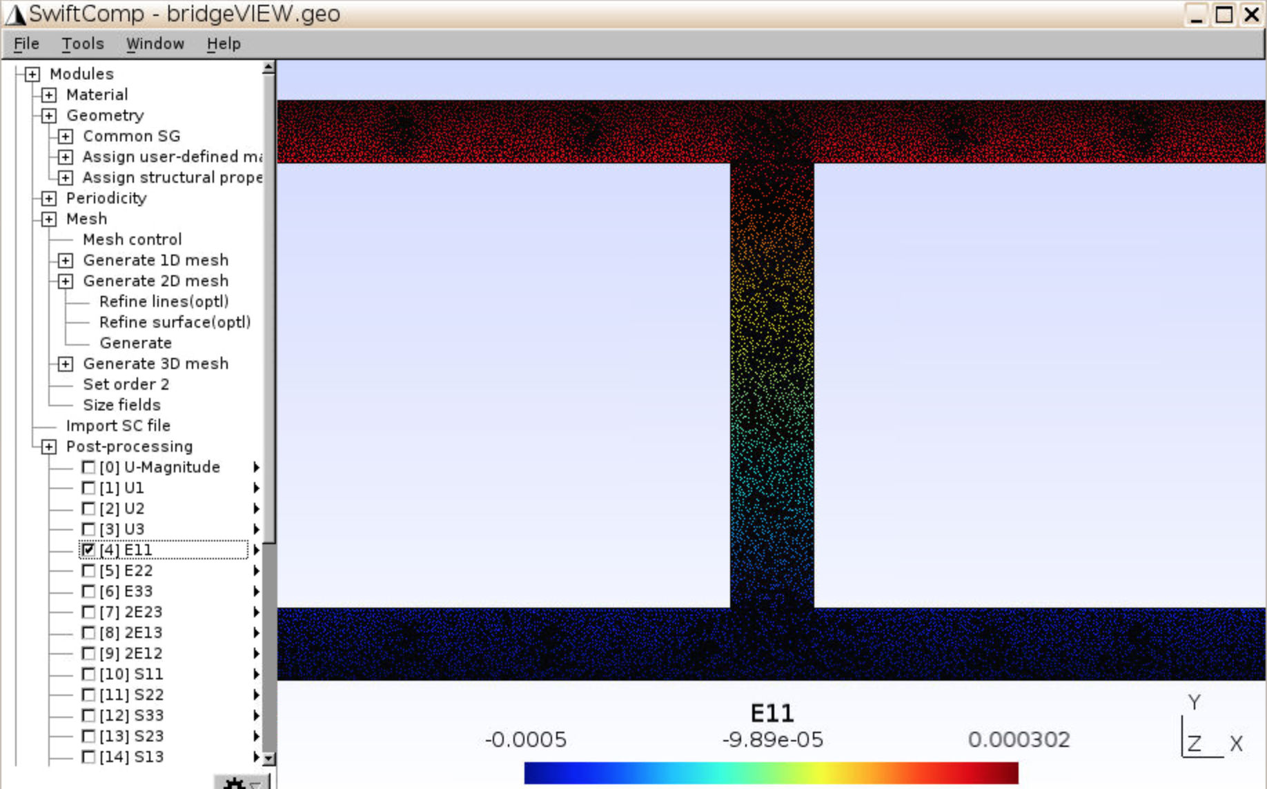
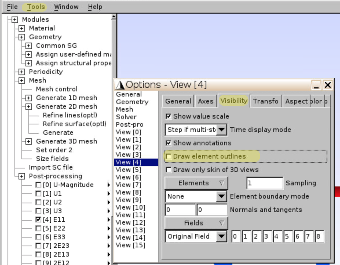
- You may uncheck the
Draw element outlinesif necessary. This would help reveal the stress distribution in steel.