Descriptions
In this wiki tutorial, you will learn about how to obtain effective properties of composites possessing four microstructures, including
- hexagonal packed fibers
- square packed fibers with interphase layer between fiber and matrix
- 0/90 laminate
- two spheres included in matrix
Geometric dimensions and material properties are taken from Challenge Problems for the Benchmarking of Micromechanics Analysis. Apart from how to calculate effective material properties of these four microstructures, you will also learn about
- how to extract and plot local stress values along a line after dehomogenization (in Case 2)
- how to draw a sphere and assign material properties by editing command files (in Case 4)
Software Used
Case 1. Hexagonal Pack Microstructure
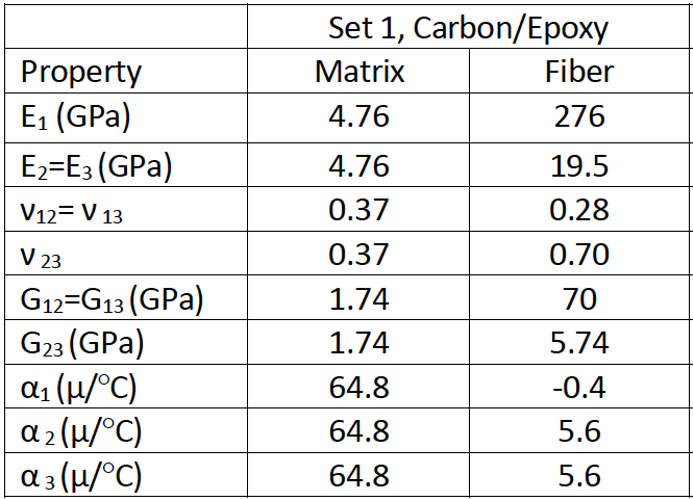
The hex pack microstructure describes a continuous fiber reinforced composite. Figure 1 shows the cross-section. Dark portion represents fiber. Volume fraction of fiber is 60%. Material properties are given in Figure 2.

Video
You may refer to the YouTube video for hex pack micromechanics analysis.
Solution Procedures
- Launch Swift Comp.
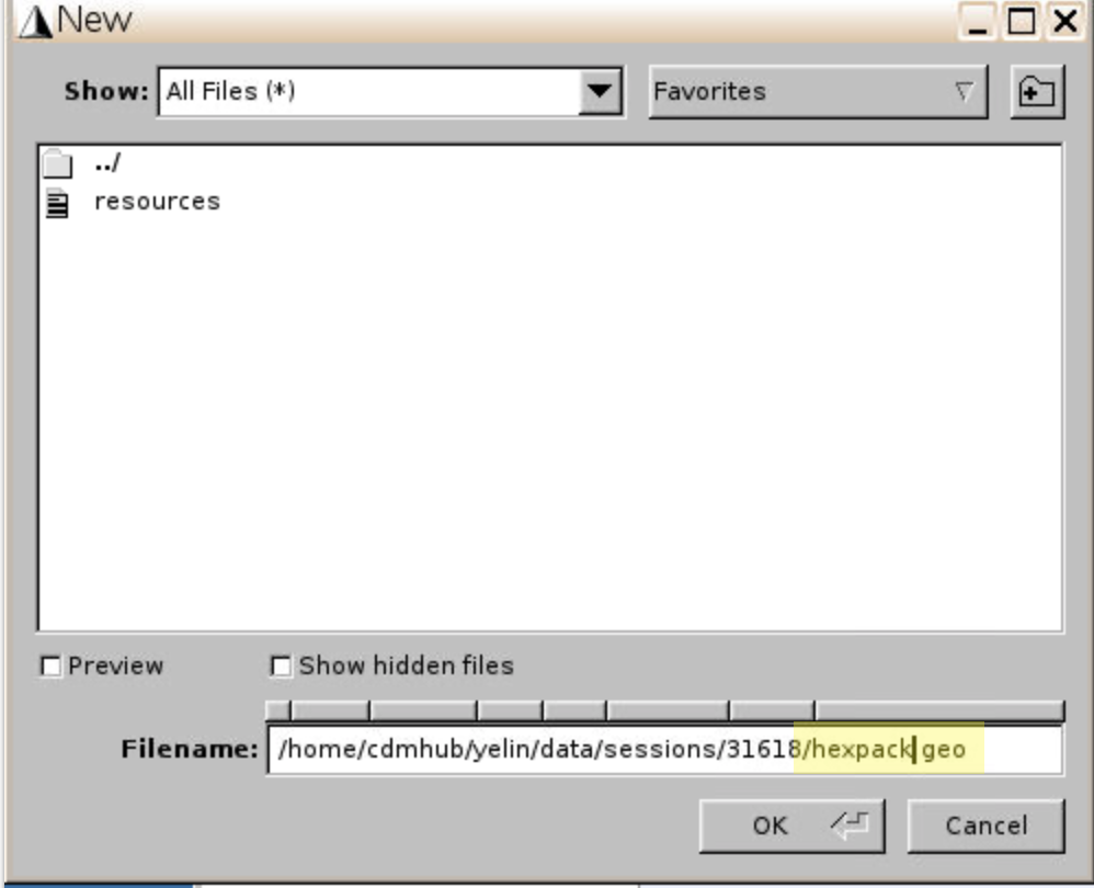
- Create a new file.
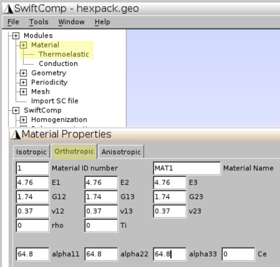
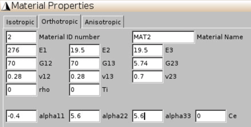
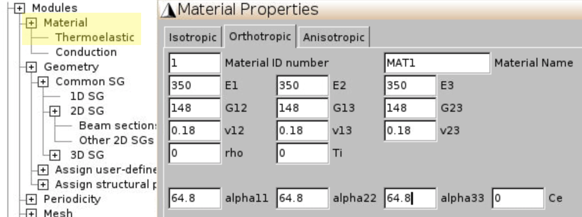
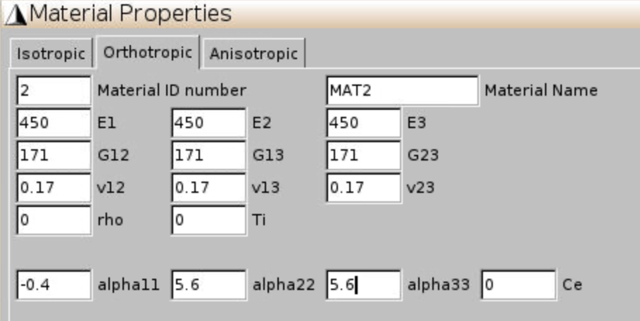
- Add material properties
- Click
Material,Thermoelastic,Orthotropic, input matrix and fiber properties given in Figure 2, clickAddfor each material. Finally clickClose.
- Click
- Define SG geometry
- Click
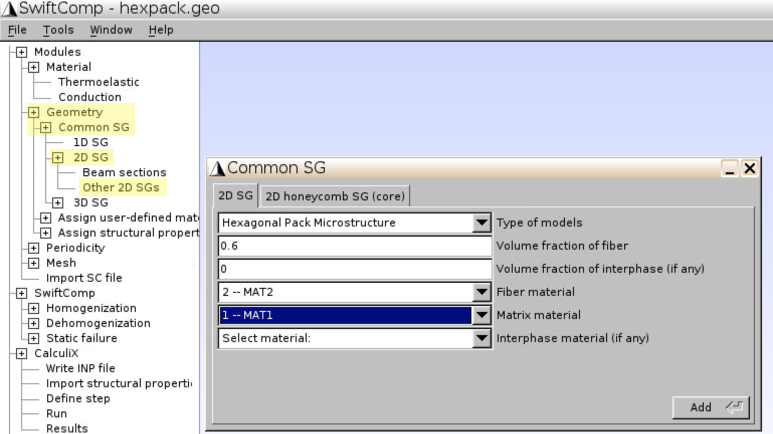
Geometry,Common SG,2D SG,Other 2D SGs. - Select Type of models:
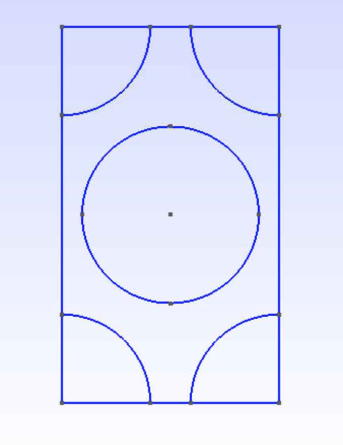
Hexagonal Pack Microstructure, input Volume fraction of fiber:0.6, select Fiber and Matrix materials to beMAT2andMAT1, clickAdd. The hex pack geometry is generated as shown in Figure 7.
- Click
- Mesh
- Click
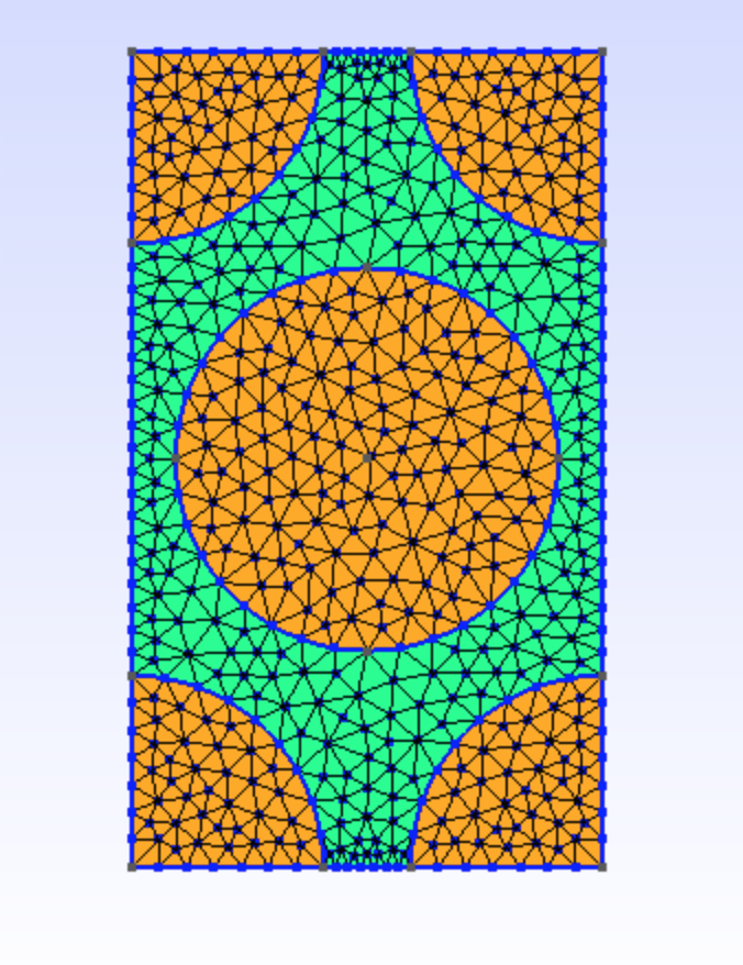
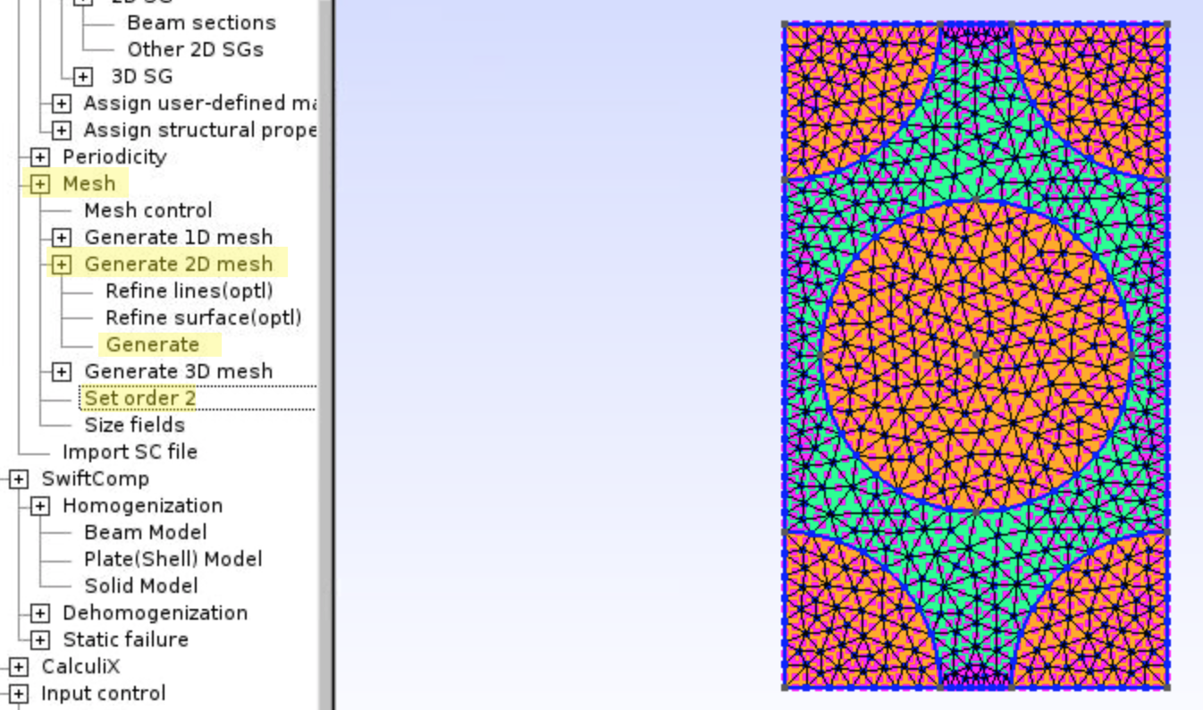
Mesh,Generate 2D mesh,Generate. - Click
Set order 2.
- Click
- Homogenization
- Click
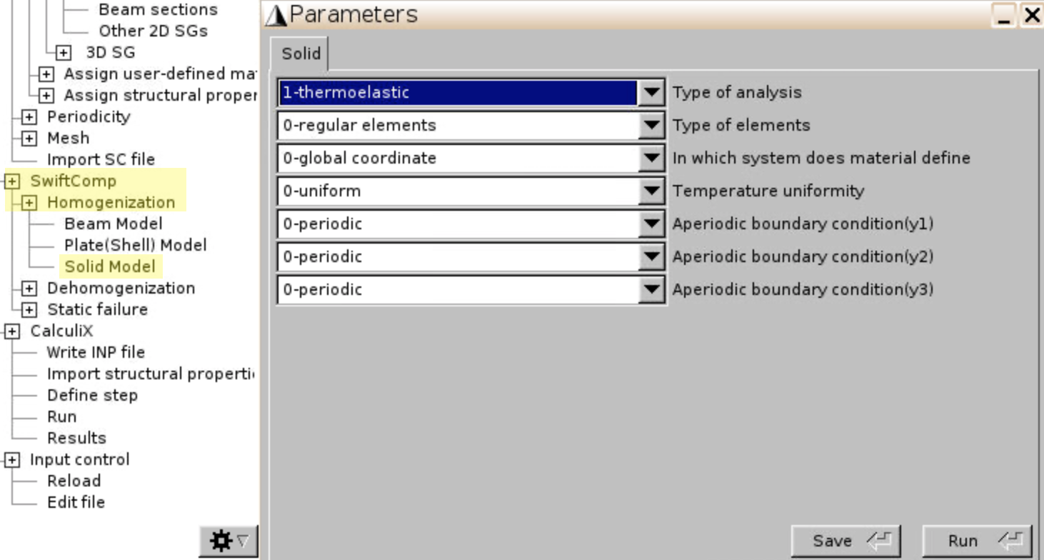
SwiftComp,Homogenization,Solid Model - Select
1-thermoelasticas Type of analysis - Click
Save,Run.

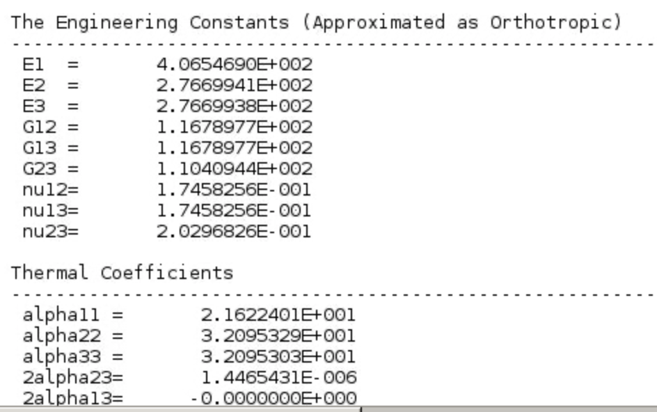
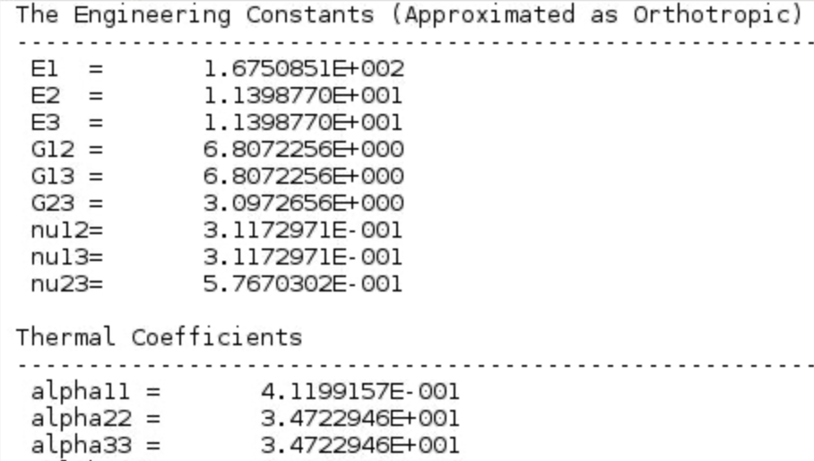
- The effective elastic properties and CTEs of the homogenized hex pack structure is given in Figure 11.

- Click
Case 2. Square Pack Microstructure
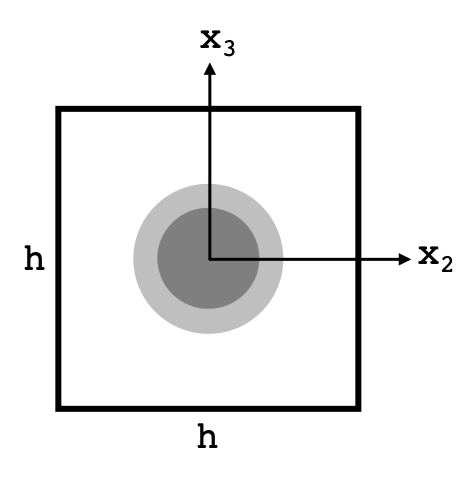
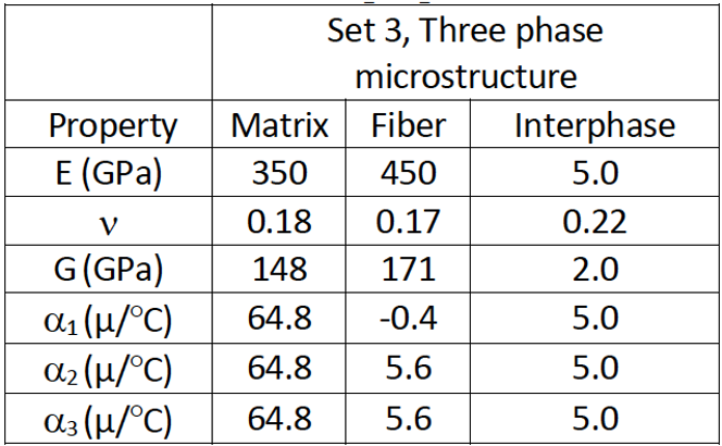
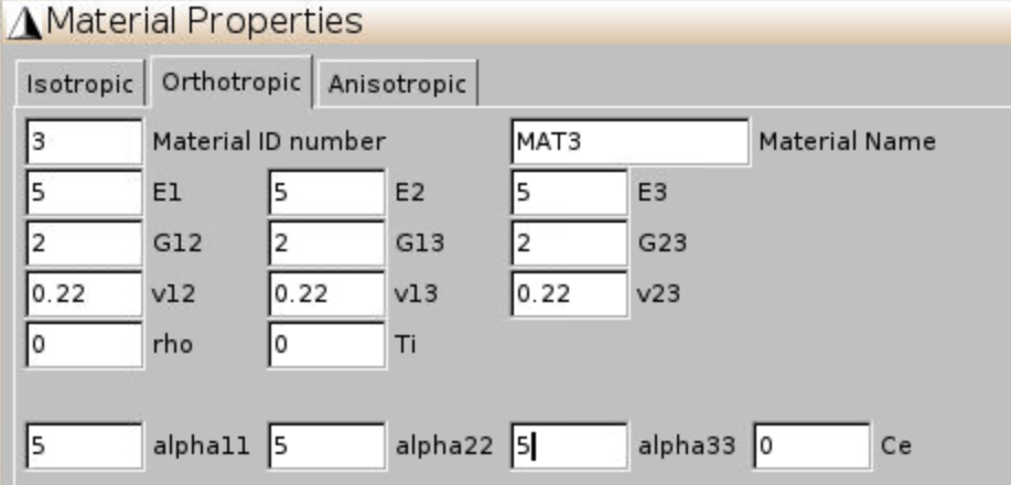
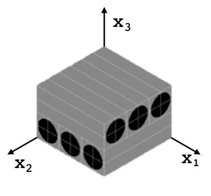
Cross section of a square pack composite with an interphase layer is given in Figure 12. Volume fraction of fiber and interphase is 60% and 1% respectively. Material properties are given in Figure 13.
Solution Procedures
- Add material properties
- Click
Material,Thermoelastic,Orthotropic, input the 3 material properties, clickAddfor each material. Finally clickClose.
- Click
- Define SG geometry
- Click
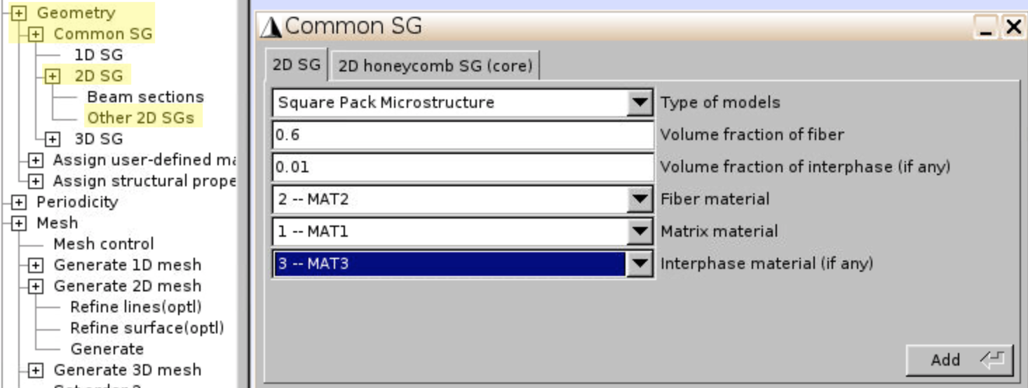
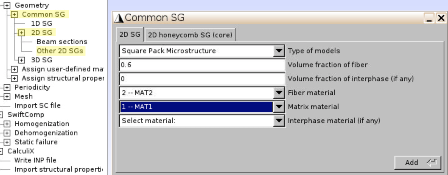
Geometry,Common SG,2D SG,Other 2D SGs. - Select Type of models:
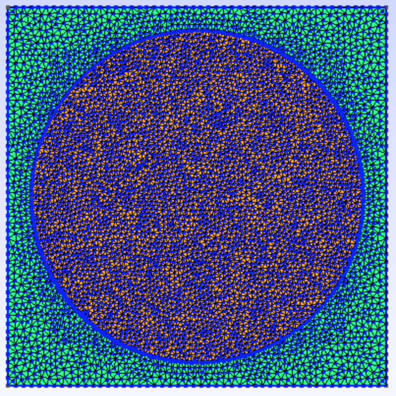
Square Pack Microstructure, input Volume fraction of fiber:0.6, Volume fraction of interphase:0.01, select materials, clickAdd. The square pack geometry is generated as shown in Figure 18.

- You may find the radii of fiber and interphase circles in
Input control,Edit file.

- Click
- Mesh
- As the interphase is very thin, we refine the mesh for circle arcs surrounding interphase layer.
- Click
Mesh,Generate 2D mesh,Refine lines. - Input Number of points:
50 - Click the 8 circle arcs.
- Press
e, andq.

- Click
Generate 2D mesh,Generate.
- Homogenization
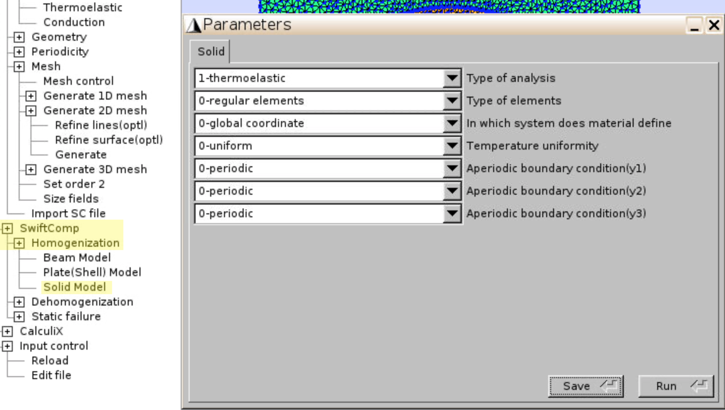
- Click
SwiftComp,Homogenization,Solid Model - Select
1-thermoelasticas Type of analysis - Click
Save,Run.
- The effective elastic properties and CTEs of the homogenized square pack structure is given in Figure 11.
- Click
- Dehomogenization
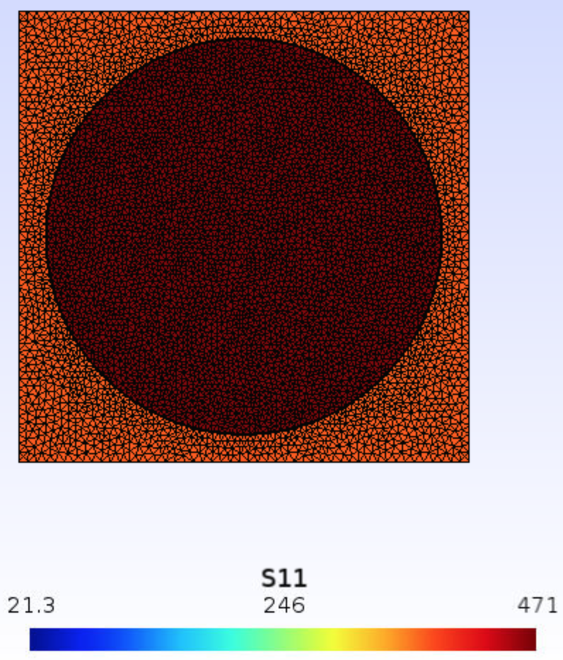
- Since we do not know the actual deformations, here we only show the representative local stress field, such as $$\sigma_{11}$$ distribution across the cross section under $$\epsilon_{11} = 1$$ loading.
- Click
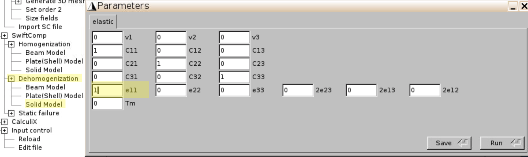
Dehomogenization,Solid Model. - Input
1for e11. - Click
Save, andRun.
- Axial stress $$\sigma_{11}$$ shows symmetric distribution across the cross section.
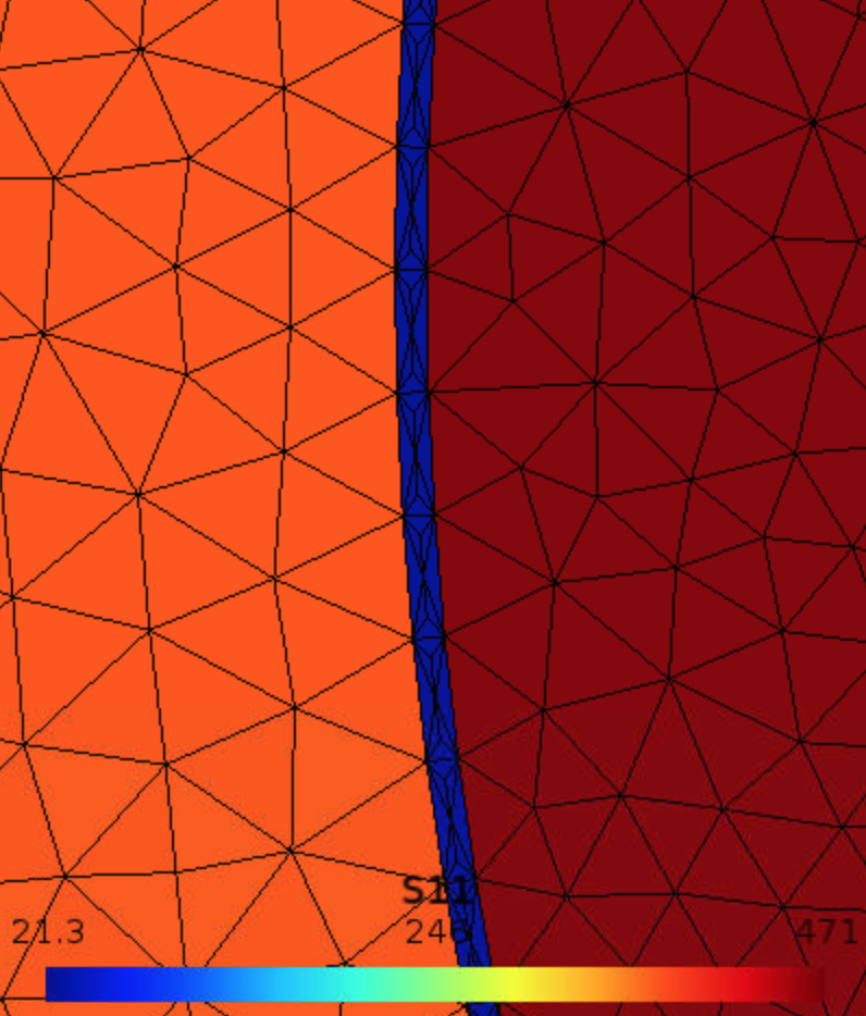
- Zoom in to check the interface layer.
- Plot $$\sigma_{11}$$ along the center line
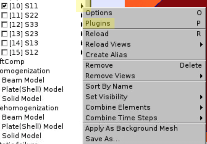
- Click the triangular arrow beside S11, click
Plugins.
- Choose
CutGridforView[10](S11) - Set (X0, Y0, Z0) =
(0, 0, 0), (X1, Y1, Z1) =(0.5, 0, 0), NumPointsU =100(or larger). This will create a cut from (0, 0, 0) to (0.5, 0, 0) using 100 points. - (X2, Y2, Z2) is set to be the same as (X0, Y0, Z0) to avoid additional points of no interest here.
- The other side, e.g., from (-0.5, 0, 0) to (0, 0, 0), is symmetric.
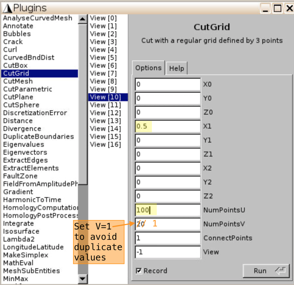
- Click
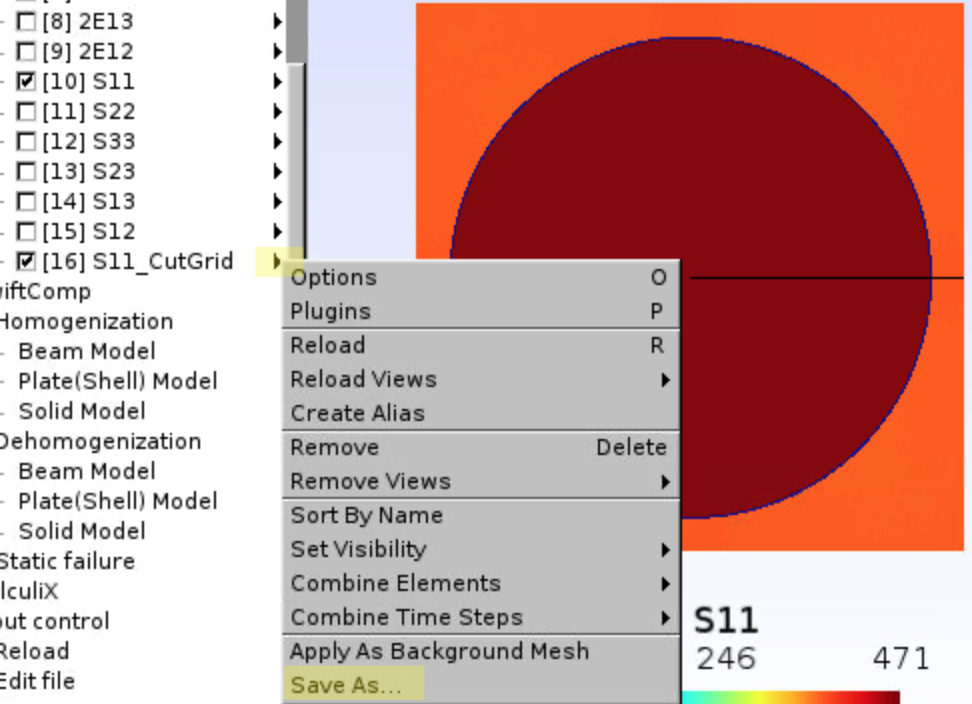
Run. You’ll see a new View calledS11_CutGrid. - Save the new view as
.txtfile by clicking the triangle arrow and chooseSave As....
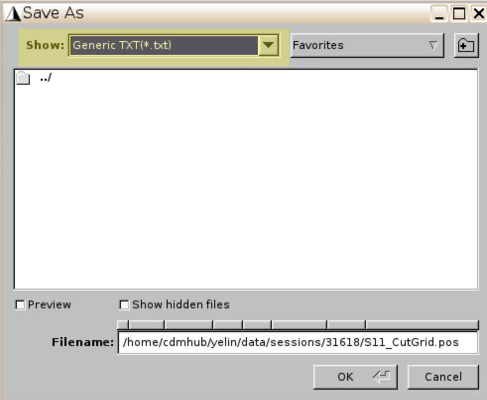
- File format is selected as
Generic TXT(*.txt), since the .txt file will only contain numbers, and is easier to be separated.
- Download the exported CutGrid file to your local computer. Open it in Excel. If you have problems about how to download, please refer to this tutorial – 2.3 Check results and save files.
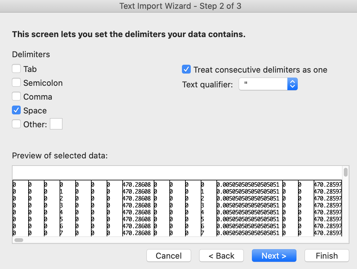
- Find the x values (in the 5th column) and corresponding s11 values (in the 8th column). Plot S11 vs. X.
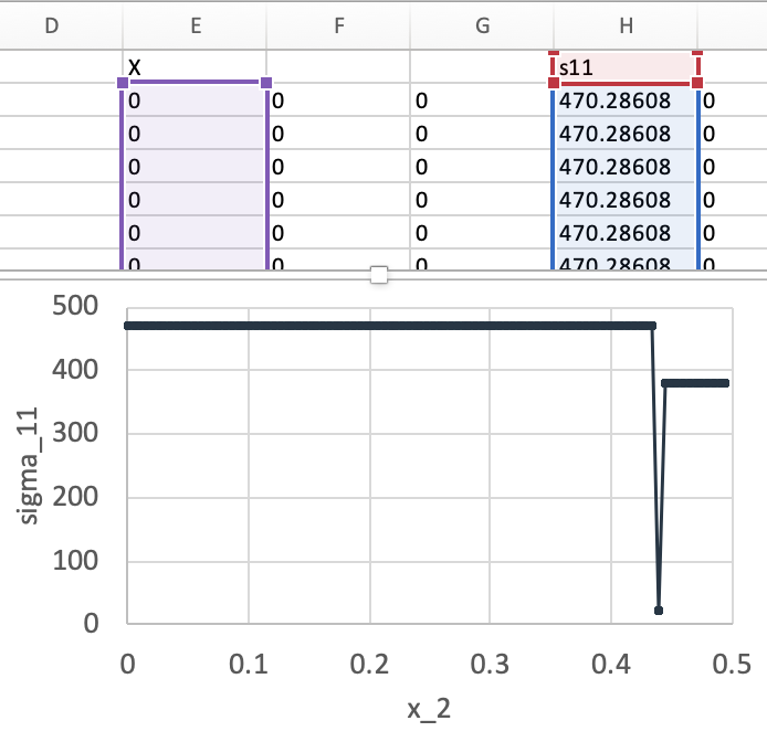
- Since the NumPointsV was set to be 20 by default, there will be 20 points of the same value. Feel free to remove duplicated values in Excel.
- It’s also good to save as other formats, such as
.poswhich is the default format. To extract (x,y,z) positions and corresponding S11 values from a .pos file, please refer to this tutorial – Dehomogenization part.
- Click the triangular arrow beside S11, click
Case 3. 0/90 Laminate
Figure 33 shows the microstructure of a 0/90 laminate.
The fiber volume fraction is 60%. Diameter of the fiber is 5 microns. Fiber and matrix properties are the same as given in Figure 2 for Case 1.
We first calculate the effective properties of lamina using square pack geometry, then input lamina properties to calculate the laminate properties.
Solution Procedures
- Calculate lamina properties
- Click
Material,Thermoelastic,Orthotropic, input matrix and fiber properties given in Figure 2, clickAddfor each material. Finally clickClose.
(Image(Fig34(1)_Mat1.png, 461px) failed - File not found) (Image(Fig34(2)_Mat2.png, 358px) failed - File not found) - Click
Geometry,Common SG,2D SG,Other 2D SGs. - Select Type of models:
Square Pack Microstructure, input Volume fraction of fiber:0.6, select Fiber and Matrix materials to beMAT2andMAT1, clickAdd.
- Click
Mesh,Generate 2D mesh,Generate, andSet order 2.

- Click
SwiftComp,Homogenization,Solid Model. Select1-thermoelastic. ClickSave,Run.
- Effective lamina properties are given in the .msh.k file.
- Click
- Input lamina properties
- Create a new .geo file for laminate.

- Click
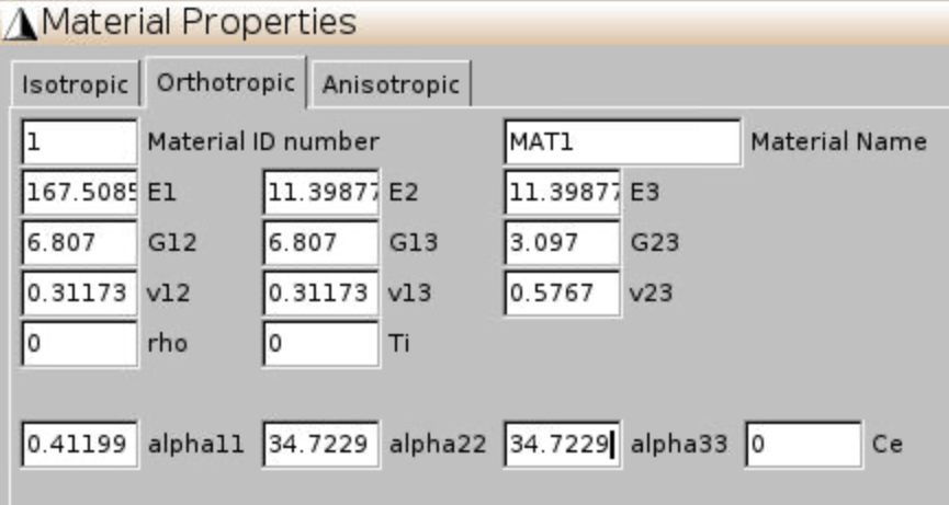
Material,Thermoelastic,Orthotropic, input lamina properties in Figure 39. ClickAddandClose.
- Create a new .geo file for laminate.
- Define SG geometry
- Click
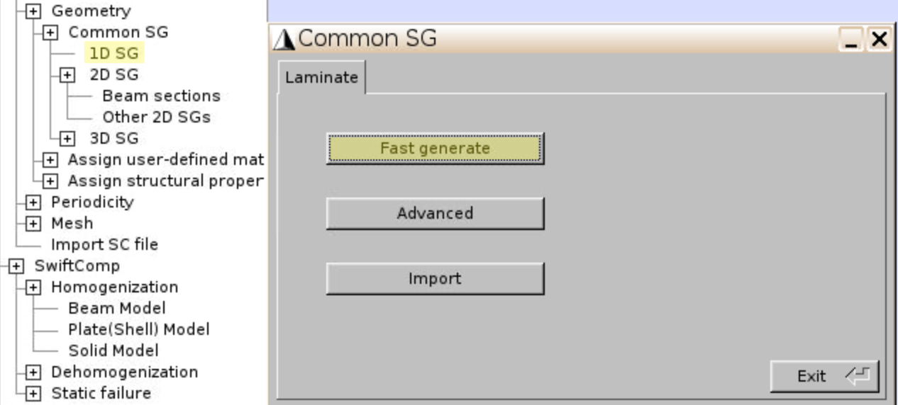
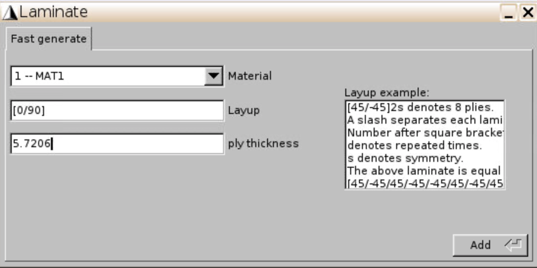
Geometry,Common SG,1D SG,Fast generate.
- Input Layup:
[0/90], ply thickness:5.7206, clickAdd. The ply thickness is calculated by the fiber volume fraction (0.6) and fiber diameter (5).

- Click
- Mesh
- Click
Mesh,Generate 1D mesh,Generate.
- Click
- Homogenization
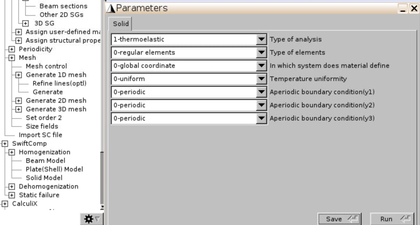
- Click
SwiftComp,Homogenization,Solid Model. Select1-thermoelastic. ClickSave,Run.
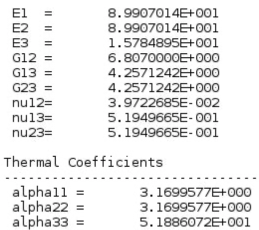
- The effective laminate properties are given in msh.k file.
- Click
Case 4. Double spherical inclusion
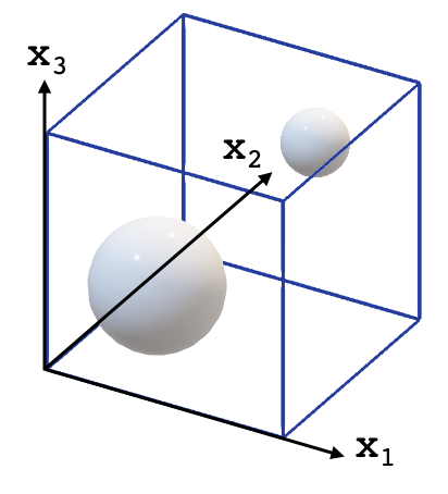
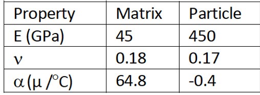
Reinforcing particles or voids in composites are represented by spheres inside a box. The double spherical inclusion microstructure is shown in Figure 46. The box is 2*2*2 microns. Diameter of the two spheres are 1 and 0.5 microns. The larger sphere is centered at (0.6, 0.6, 0.6) and the smaller sphere is centered at (1.5, 1.7, 1.3). Material properties are given in Figure 47.
Solution Procedures
- Add material properties
- Click
Material,Thermoelastic, input matrix and fiber properties given in Figure 47, clickAddfor each material. Finally clickClose.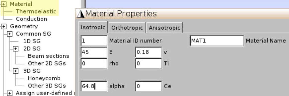

- Click
- Define SG geometry
- SwiftComp already coded the single spherical inclusion microstructure as one of the common SGs. Here we first create one sphere, and edit the commands to create the second sphere.
- Alternatively, you may download !Gmsh 2.9.3 from http://gmsh.info//bin/, draw the two spheres, and copy the commands into the .geo file on cdmhub.
- To create an arbitrary spherical inclusion microstructure, click
Geometry,Common SG,3D SG,Other 3D SGs. SelectSpherical Inclusions Microstructure, input any number as Volume fraction as we will change the radius later.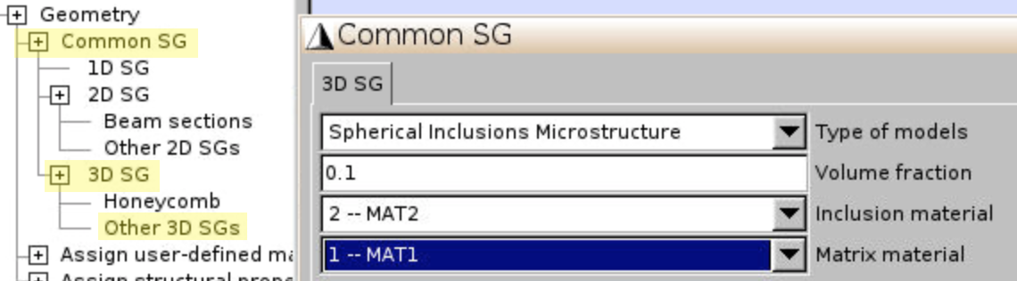
- Click
Input control,Edit file.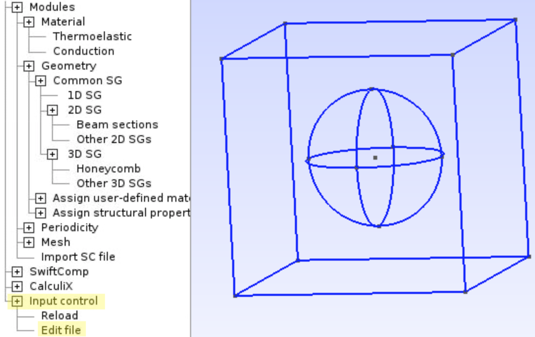
- You’ll find the commands that describes the geometry starting from Point (1).
- Modify the cubic box
 (old commands)
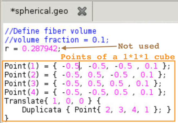
- Points are formatted as
Point(#) = {x,y,z, mesh size}. - Points (1), (2), (3), (4) define a 1*1 square at x = -0.5, which is the left face of the 1*1*1 cube.
- Translate of the four points by x+1 to x = 0.5, to get the other four points on the right face of the 1*1*1 cube.
- The eight points represent a 1*1*1 cube from (-0.5, -0.5, -0.5) to (0.5, 0.5, 0.5)
 (new commands)
- Now change the (x,y,z) numbers so that the cube is 2*2*2, from (0, 0, 0) to (2, 2, 2).
- Change the mesh size to be 1.
- Change the Translate distance to be 2.
- Points are formatted as
- Modify the larger sphere
 (old commands)
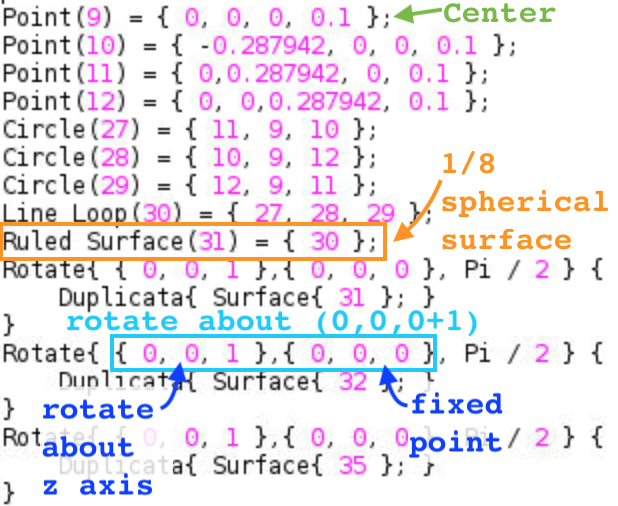
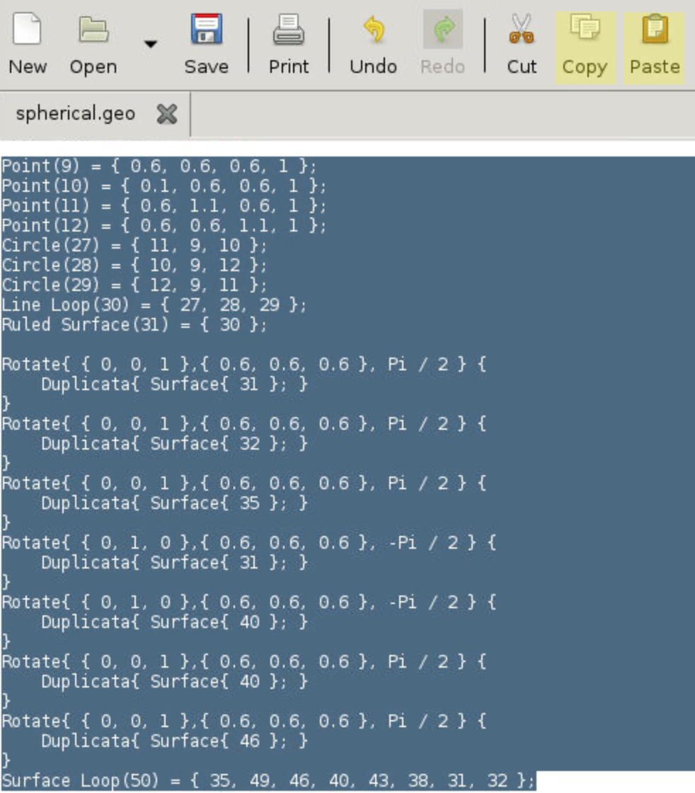
- A 1/8 sphere is defined by 4 points, 3 arcs, and 1 surface. The surface is then rotated 7 times to create the entire sphere.
 (new commands)
- Change the (x,y,z) of Point (9) so that the sphere is centered at (0.6, 0.6, 0.6).
- Points on the surface are (center point +/- radius). The radius of the larger sphere is 0.5.
- Mesh size is changed to 1 again.
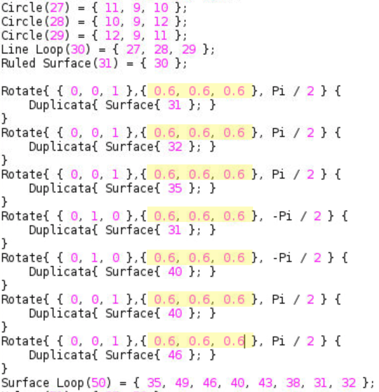 (new commands)
- Center of rotation should be the spherical center (0.6, 0.6, 0.6).
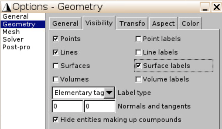
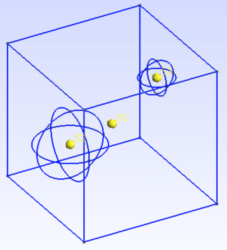
- Check the geometry in SwiftComp by clicking
Input control,Reload. Feel free to add or remove visible labels in Options.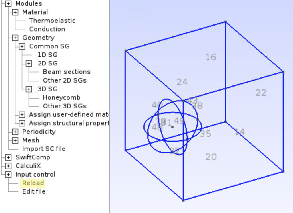
- A 1/8 sphere is defined by 4 points, 3 arcs, and 1 surface. The surface is then rotated 7 times to create the entire sphere.
- Create the smaller sphere
- Select the commands that create the larger sphere, copy and paste.
- Change element numbers and (x,y,z) values.
- To avoid error caused by dummy element number, I did not follow a sequential order, but just changed Point(n) into Point(n+40), and changed Line(m) into Line(m+30). Surfaces are in the same sequence as Lines.
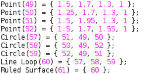

- For example, Point(9) is changed into Point(49), Circle(27) is changed into Circle(57). Circle means circle arc which is a line element.
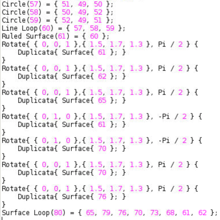
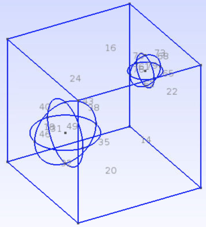
- Rotation center should be the spherical center (1.5, 1.7, 1.3). All element numbers in Figure 62 are lines or surfaces, and are changed from m to m+30.
- Select the commands that create the larger sphere, copy and paste.
- Assign material properties
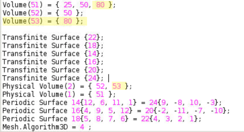
- Volume(51) is the non-particle space (matrix). Volume(51) = {25, 50} means the outer surface is Surface(25) (the cubic box), while the inner hole is Surface(50) (the larger sphere). Add
80at the end as another inner surface to exclude the small sphere from matrix. - Add a new volume for the small sphere.
- Physical volume (2) is the particle. Add the small sphere. This would assign particle properties to the small sphere.
- Volume(51) is the non-particle space (matrix). Volume(51) = {25, 50} means the outer surface is Surface(25) (the cubic box), while the inner hole is Surface(50) (the larger sphere). Add
- Mesh
- Click
Mesh,Generate 3D mesh,Generate, andSet order 2.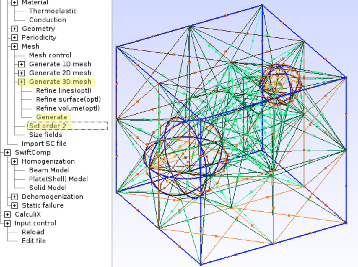
- Click
- Homogenization
- Click
SwiftComp,Homogenization,Solid Model. Select1-thermoelastic. ClickSave,Run.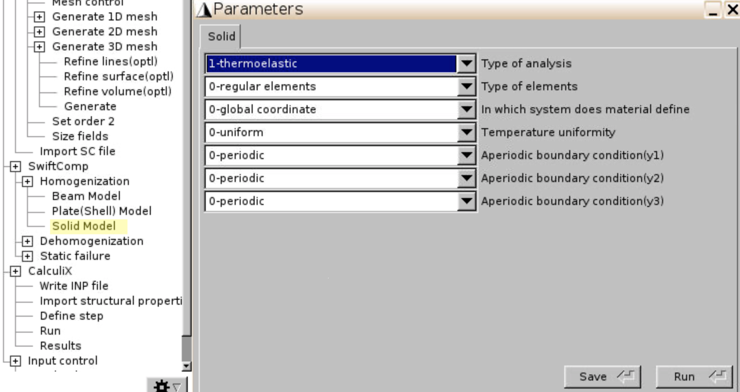
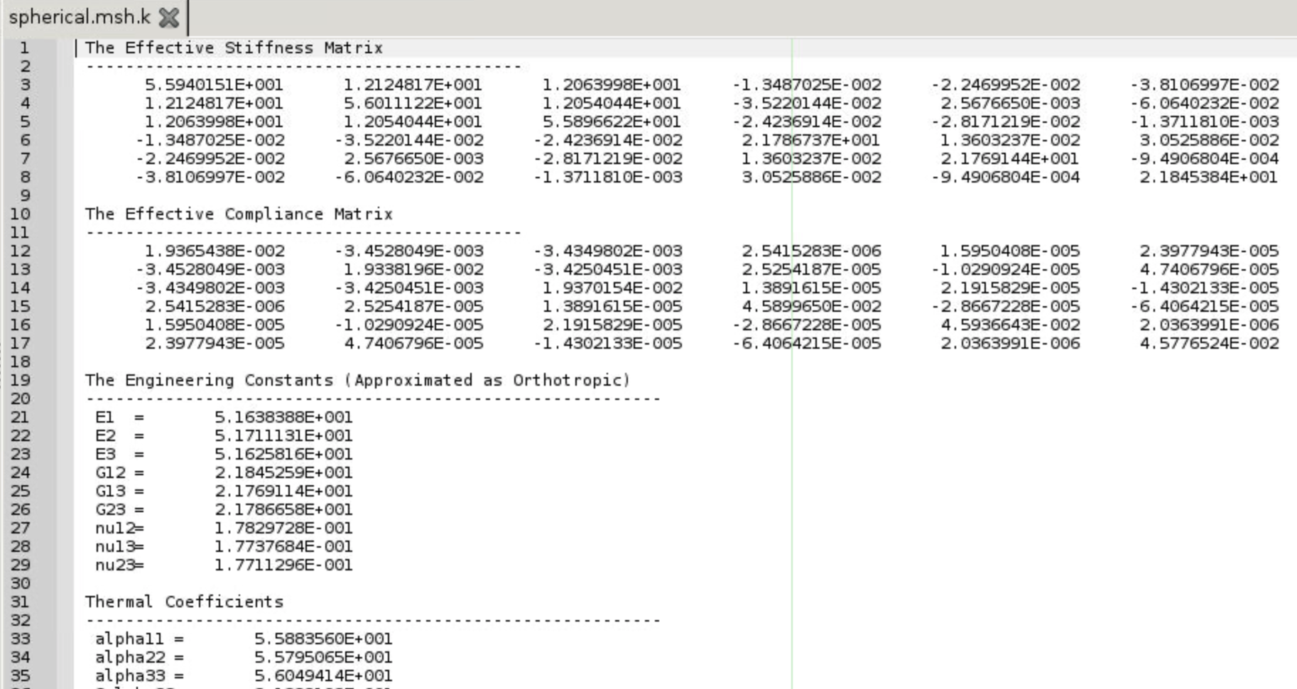
- The effective properties are given in .msh.k file.
- Click
References
- Andrew J Ritchey; Hamsasew Sertse; Johnathan Goodsell; Wenbin Yu; Byron Pipes (2015), “Micromechanics Simulation Challenge Level I Results,” https://cdmhub.org/resources/948.
- Xin Liu; Wenbin Yu (2017), “Gmsh4SC USER’S MANUAL”, https://cdmhub.org/resources/1342/download/Gmsh4SCManual.pdf